<?xml version="1.0" encoding="utf-8"?><feed xmlns="http://www.w3.org/2005/Atom" xml:lang="en-us, es_ES"><generator uri="https://jekyllrb.com/" version="3.10.0">Jekyll</generator><link href="https://vladislav-morozov.eu/feed.xml" rel="self" type="application/atom+xml" /><link href="https://vladislav-morozov.eu/" rel="alternate" type="text/html" hreflang="en-us, es_ES" /><updated>2026-07-23T20:56:48+00:00</updated><id>https://vladislav-morozov.eu/feed.xml</id><title type="html">Vladislav Morozov, PhD</title><subtitle>Vladislav Morozov, PhD | Data Science and Statistics 
</subtitle><author><name>Vladislav Morozov</name><email>vladislav.morozov [at] barcelonagse.eu</email></author><entry><title type="html">Introducing unit-averaging</title><link href="https://vladislav-morozov.eu/blog/statistics/machine%20learning/2025-09-28-unit-averaging-released/" rel="alternate" type="text/html" title="Introducing unit-averaging" /><published>2025-09-28T00:00:00+00:00</published><updated>2025-09-28T00:00:00+00:00</updated><id>https://vladislav-morozov.eu/blog/statistics/machine%20learning/unit-averaging-released</id><content type="html" xml:base="https://vladislav-morozov.eu/blog/statistics/machine%20learning/2025-09-28-unit-averaging-released/"><![CDATA[<script type="text/x-mathjax-config">
MathJax.Hub.Config({
 "HTML-CSS": { linebreaks: { automatic: true } },
         SVG: { linebreaks: { automatic: true } }
});
</script>

<script type="text/javascript">
if (window.MathJax) {
  MathJax.Hub.Queue(
    ["Typeset",MathJax.Hub]
  );
}
</script>

<p>I’ve released version 1.0 of <code class="language-plaintext highlighter-rouge">unit-averaging</code>, a Python package for
efficient ensemble estimation of unit-specific parameters in
heterogeneous data! It’s now available on
<a href="https://pypi.org/project/unit-averaging/">PyPI</a> with full
<a href="https://vladislav-morozov.github.io/unit-averaging/">documentation on my
web</a>. The package
automates optimal weighting, supports flexible workflows, and integrates
easily into existing pipelines. In this post, I briefly outline the
problem it addresses, the approach, and how to use the package.</p>

<!--more-->

<ul id="markdown-toc">
  <li><a href="#the-problem-estimating-individual-parameters" id="markdown-toc-the-problem-estimating-individual-parameters">The Problem: Estimating Individual Parameters</a></li>
  <li><a href="#solution-unit-averaging" id="markdown-toc-solution-unit-averaging">Solution: Unit Averaging</a></li>
  <li><a href="#the-package" id="markdown-toc-the-package">The Package</a></li>
  <li><a href="#next-steps" id="markdown-toc-next-steps">Next Steps</a></li>
</ul>

<h2 id="the-problem-estimating-individual-parameters">The Problem: Estimating Individual Parameters</h2>

<p>Let’s start with a motivating example. Imagine you want to forecast
Spain’s gross domestic product (GDP) for next year. You have panel data
for Spain and other European countries. How do you construct an
<em>efficient</em> forecast?</p>

<p>There are two obvious options:</p>

<ul>
  <li>Build your forecast using only Spanish data.</li>
  <li>Pool all the data and fit a single predictive model.</li>
</ul>

<p>Neither is ideal. The first option is less biased but has higher
variance and ignores most of the data. The second option likely
introduces high bias, especially if the model is nonlinear or dynamic,
since different countries have different economic dynamics.</p>

<p>This example illustrates a general problem: estimating unit-specific
parameters (e.g., GDP forecasts for Spain) from a panel of units, each
with its own version of the parameter (the problem of unobserved
heterogeneity).</p>

<h2 id="solution-unit-averaging">Solution: Unit Averaging</h2>

<p><code class="language-plaintext highlighter-rouge">unit-averaging</code> offers a compromise third solution called <em>unit
averaging</em> that Christian Brownlees and I develop in a <a href="https://arxiv.org/abs/2210.14205">paper of
ours</a>. Unit averaging uses an ensemble
of unit-level estimators.  Such an ensemble can exploit panel-wide information 
to optimally reduce variance while controlling bias. 
The approach works for both nonlinear and dynamic models.</p>

<p>To explain the essential idea, let \(i=1, \dots, N\) be the different
units in your data (countries, customers, firms; or studies in a
meta-analysis). The data is <em>heterogeneous</em> in the sense that each unit
\(i\) has their own version of some parameter \(\theta_i\).</p>

<p>We are interested in the <em>unit-specific</em> “focus parameter”
\(\mu(\theta_i)\) for some fixed unit \(i\). This parameter could be
predictive (e.g., GDP forecast, churn probability) or causal/structural
(e.g., individual treatment effects, multipliers). 
The focus function \(\mu(\cdot)\) can also depend on the data of the target unit.</p>

<p>The goal is to estimate \(\mu(\theta_i)\) optimally, minimizing mean
squared error (MSE).</p>

<p>The unit averaging approach has two steps:</p>

<ol>
  <li>Estimate each \(\theta_i\) with the individual (or unit-specific)
estimator \(\hat{\theta}_i\). Compute \(\mu(\hat{\theta}_i)\) for all
\(i\).</li>
  <li>Compute a weighted average of the individual estimators:</li>
</ol>

\[\hat{\mu}(\mathbf{w}) = \sum_{i=1}^N w_i \mu(\hat{\theta}_i),\]

<p>where the weights \(\mathbf{w} = (w_1, \dots, w_N)\) are non-negative and
sum to 1.</p>

<p>To understand the intuition behind \(\hat{\mu}(\mathbf{w})\), suppose that
we can write the individual-specific true parameters \(\theta_i\) as a sum
of two pieces:</p>

\[\theta_i = \mathbb{E}[\theta_i] + \eta_i.\]

<p>Here</p>

<ul>
  <li>\(\mathbb{E}[\theta_i]\) is the average value that is <em>common</em> to all
units (e.g. broad global economic laws).</li>
  <li>\(\eta_i\) is a mean-zero value that is <em>specific</em> to unit \(i\)
(e.g. Spain-specific dynamics).</li>
</ul>

<p>Unit averaging is motivated by the fact that each unit carries
information about \(\mathbb{E}[\theta_i]\). Using data on non-target units
may help reduce the uncertainty about \(\mathbb{E}[\theta_i]\) and reduce
the overall variance of the estimator. By averaging
\(\mu(\hat{\theta}_i)\) after estimation (not pooling data beforehand),
unit averaging can exploit shared information across units without
assuming a specific model form.</p>

<h2 id="the-package">The Package</h2>

<p><code class="language-plaintext highlighter-rouge">unit-averaging</code> is a lightweight Python I wrote to implement unit
averaging. It implement all the schemes \(\hat{\mu}(\mathbf{w})\) that we
propose, including the MSE-optimal weights. I tried to design it with a
few goals in mind:</p>

<ul>
  <li>Flexibility: the package works with panel data, meta-analysis, and
other heterogeneous datasets.</li>
  <li>Versatility: the implemented averagers are compatible with standard
estimation packages for constructing \(\hat{\theta}_i\); minimal code
changes required.</li>
  <li>Speed: optimal weights are near-instant to compute even with tens of
thousands of units thanks to using <code class="language-plaintext highlighter-rouge">cvxpy</code> in the background.</li>
  <li>Customization: if the built-in schemes don’t fit your needs, you can
implement your own weighting logic by subclassing the base classes.</li>
</ul>

<p>I also tried to keep the interface simple and uniform. One should need
just three line to integrate any unit averager into a pipeline that
already runs individual estimators \(\hat{\theta}_i\): importing the
averager class, instantiating it, and fitting the instance. 
For example, if you already have the individual-specific <code class="language-plaintext highlighter-rouge">estimates</code>
(along with their matrices of <code class="language-plaintext highlighter-rouge">covariances</code>), you can run 
optimal unit averaging as</p>

<div class="language-python highlighter-rouge"><div class="highlight"><pre class="highlight"><code><span class="kn">from</span> <span class="nn">unit_averaging</span> <span class="kn">import</span> <span class="n">OptimalUnitAverager</span>

<span class="n">averager</span> <span class="o">=</span> <span class="n">OptimalUnitAverager</span><span class="p">(</span>
    <span class="n">focus_function</span><span class="o">=</span><span class="n">parameter_of_interest</span><span class="p">,</span>      <span class="c1"># focus function
</span>    <span class="n">ind_estimates</span><span class="o">=</span><span class="n">estimates</span><span class="p">,</span>                   <span class="c1"># individual estimates
</span>    <span class="n">ind_covar_ests</span><span class="o">=</span><span class="n">covariances</span>                 <span class="c1"># individual covariances
</span><span class="p">)</span>

<span class="n">averager</span><span class="p">.</span><span class="n">fit</span><span class="p">(</span><span class="n">target_id</span><span class="o">=</span><span class="s">"unit_of_interest"</span><span class="p">)</span>
</code></pre></div></div>

<p>After fitting, the computed \(\hat{\mu}(\mathbf{w})\) is available in the
<code class="language-plaintext highlighter-rouge">estimate</code> attribute, ready for downstream use in place of the original
unit-specific estimate.</p>

<p>Finally, the averager also stores the fitted weights in the <code class="language-plaintext highlighter-rouge">weights</code>
attributes. Those weights can be interesting in themselves, as they can
sometimes reveal patterns in the data that are driven by similarities in
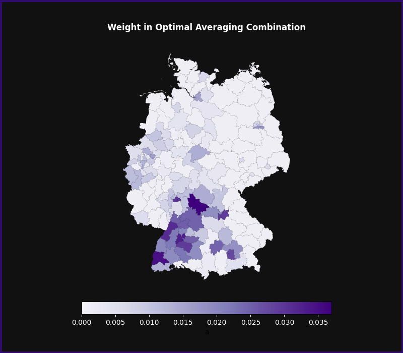
the focus parameters between units. For example, when predicting
unemployment in Frankfurt using data from other German regions, optimal
unit averaging assigns higher weights to nearby regions and other major
cities like Munich and Hamburg (see <a href="https://vladislav-morozov.github.io/unit-averaging/tutorials/plot_1_basics.html">this tutorial</a> for details).</p>

<p><img src="https://vladislav-morozov.github.io/unit-averaging/_images/sphx_glr_plot_1_basics_001.png" alt="Frankfurt map" /></p>

<h2 id="next-steps">Next Steps</h2>

<p>Check out:</p>

<ul>
  <li>The <a href="https://arxiv.org/abs/2210.14205">original paper</a> for full details.</li>
  <li>The <a href="https://vladislav-morozov.github.io/unit-averaging/tutorials/plot_1_basics.html">Getting Started</a> tutorial for an end-to-end example of unit averaging.</li>
  <li>The <a href="https://vladislav-morozov.github.io/unit-averaging/reference/index.html">API documentation</a> for the various averager classes available.</li>
</ul>]]></content><author><name>Vladislav Morozov</name><email>vladislav.morozov [at] barcelonagse.eu</email></author><category term="Statistics" /><category term="Machine Learning" /><category term="Python" /><summary type="html"><![CDATA[`unit-averaging`: A package for unit averaging in Python. Efficient ensemble estimation of unit-specific parameters]]></summary><media:thumbnail xmlns:media="http://search.yahoo.com/mrss/" url="https://vladislav-morozov.eu/assets/img/blog/ua-pkg.png" /><media:content medium="image" url="https://vladislav-morozov.eu/assets/img/blog/ua-pkg.png" xmlns:media="http://search.yahoo.com/mrss/" /></entry><entry><title type="html">How to Stand Out in a Master’s in Economics Application?</title><link href="https://vladislav-morozov.eu/blog/economics/2025-09-04-how-to-stand-out-econ-master/" rel="alternate" type="text/html" title="How to Stand Out in a Master’s in Economics Application?" /><published>2025-09-04T00:00:00+00:00</published><updated>2025-09-04T00:00:00+00:00</updated><id>https://vladislav-morozov.eu/blog/economics/how-to-stand-out-econ-master</id><content type="html" xml:base="https://vladislav-morozov.eu/blog/economics/2025-09-04-how-to-stand-out-econ-master/"><![CDATA[<script type="text/x-mathjax-config">
MathJax.Hub.Config({
 "HTML-CSS": { linebreaks: { automatic: true } },
         SVG: { linebreaks: { automatic: true } }
});
</script>

<script type="text/javascript">
if (window.MathJax) {
  MathJax.Hub.Queue(
    ["Typeset",MathJax.Hub]
  );
}
</script>

<p>The key issue for admissions for competitive economics master’s programs is that there are more qualified applicants than available spots. Most candidates have strong grades in economics and math. So if you want to get in a master’s and already have good grades, what can you do to distinguish yourself?</p>

<p>The answer is to show evidence of <em>deeper interest</em> in economics. People who demonstrate this through tangible work (research, writing, or technical projects) consistently stand out. This trend seems to hold both in my stint on the relevant committee and in the work of friends at other institutions.</p>

<p>As a result, I decided to write a post on some possible signals, why they matter, and how applicants can incorporate them.</p>

<!--more-->

<ul id="markdown-toc">
  <li><a href="#the-signal-problem-in-admissions" id="markdown-toc-the-signal-problem-in-admissions">The Signal Problem in Admissions</a></li>
  <li><a href="#effective-signals-in-applications" id="markdown-toc-effective-signals-in-applications">Effective Signals in Applications</a>    <ul>
      <li><a href="#undergraduate-research-work-or-independent-projects" id="markdown-toc-undergraduate-research-work-or-independent-projects">Undergraduate Research, Work, or Independent Projects</a></li>
      <li><a href="#writing-on-economic-or-data-topics" id="markdown-toc-writing-on-economic-or-data-topics">Writing on Economic or Data Topics</a></li>
      <li><a href="#technical-projects-with-economic-applications" id="markdown-toc-technical-projects-with-economic-applications">Technical Projects with Economic Applications</a></li>
    </ul>
  </li>
  <li><a href="#common-questions" id="markdown-toc-common-questions">Common Questions</a></li>
  <li><a href="#conclusion" id="markdown-toc-conclusion">Conclusion</a></li>
</ul>

<h2 id="the-signal-problem-in-admissions">The Signal Problem in Admissions</h2>

<p>There are two reasons why admissions cannot just be based purely on grades:</p>

<ol>
  <li>Grading inconsistencies: the admissions committee cannot have encyclopedic knowledge of every university’s grading standards. A 90% GPA from Institution A might mean something very different from a 90% at Institution B.</li>
  <li>Limitations of prestige: coming from a more prestigious institution with known high standards helps, but there aren’t that many of those by definition, and access to those is very uneven geographically.</li>
</ol>

<p>As a result, there typically is a large pool of applications who have “reasonable” grades from “reasonable” places.</p>

<h2 id="effective-signals-in-applications">Effective Signals in Applications</h2>

<p>So how do you distinguish yourself if you are in that pool? By sending other signals! Of this, the most useful ones:</p>

<ol>
  <li>Are <em>concrete</em> (e.g., a project, a written analysis, code).</li>
  <li>Demonstrate <em>initiative</em> (self-directed or minimally guided work).</li>
  <li>Align with <em>skills used in economics</em> (quantitative reasoning, data analysis, clear communication, programming).</li>
  <li>Verifiable: the paper PDFs, blog posts, GitHub repos all exist, are accessible and timestamped.</li>
</ol>

<p>These are not arbitrary requirements but reflections of competencies that matter in both graduate study and professional economic work.</p>

<p>There are many possible examples of such signals, and I now discuss a few of those that are useful for a <em>non-research</em> master in economics. At least some of them should be broadly accessible to anyone in an economics (or adjacent) program.</p>

<p class="note" title="Warning">These signals and recommendations are by no mean absolute, of course.</p>

<h3 id="undergraduate-research-work-or-independent-projects">Undergraduate Research, Work, or Independent Projects</h3>

<p>Perhaps the most obvious example are different kinds of research and work experience in economics and business. This may take many forms:</p>

<ul>
  <li>A research assistant (RA) position.</li>
  <li>Economist positions at a “relevant” institution (think tank, central bank, ministry, international organization, etc.).</li>
  <li>Data-related position with defined contributions.</li>
  <li>Even a course project developed into a working paper.</li>
</ul>

<p>These are fairly straightforward to include on a CV. Work experience can be listed in the relevant CV section. Moreover, team and project leaders may often be used as a reference in an application, if the program requires several letters. Independent papers should be listed on the CV with a link to an accessible PDF, along with a brief description.</p>

<p>I tend to pay attention to these things, particularly to papers. If they are broadly competently done (within their scope) and presented clearly, then it sends an impressive signal.</p>

<p class="note" title="Note">There is no expectation of groundbreaking originality and immense technical skills (if one has them, maybe a non-research master in economics is not the best fit anyway). Just something competent and at least to some extent original (possibly in just applying someone’s kind of analysis to a new country, say). The project also does not have to published (and if it is, ideally not in a predatory journal).</p>

<h3 id="writing-on-economic-or-data-topics">Writing on Economic or Data Topics</h3>

<p>Another useful signal is written work on economics outside of course assignments. Good writing demonstrates both economic understanding and communication skills. Effective examples include:</p>

<ul>
  <li>Blog posts or articles analyzing economic issues (of micro or macro nature), whether theoretically or with data.</li>
  <li>Op-eds or contributions to student publications and newspapers.</li>
</ul>

<p>This can again be linked in the CV, and people take a look at stuff that seems relevant.</p>

<p>Whether the writing makes a good impression depends on following:</p>

<ul>
  <li>Consistency: not just three LLM-written posts uploaded in the week before submitting the application.</li>
  <li>Evidence-based arguments: evidence-based arguments that show flexibility when faced with contrary evidence</li>
  <li>Relevance: Topics need not be groundbreaking, but should demonstrate economic and/or statistical reasoning.</li>
</ul>

<p>I personally like those that apply microeconomics tools (e.g. tools from intermediate micro, information econ, etc.) to some applied life scenarios. Given my background, I would also enjoy posts on computational or statistical topics, though I have not seen any examples in the wild yet.</p>

<h3 id="technical-projects-with-economic-applications">Technical Projects with Economic Applications</h3>

<p>Projects combining economics with technical skills (e.g., coding, data visualization) are also great. Observed examples:</p>

<ul>
  <li>A well-done dashboard visualizing certain economic and social changes in the applicant’s city in the context of some big reforms.</li>
  <li>A data-scraping project answering an economic question.</li>
  <li>Coordinating collection and access to a particular kind of local data resources.</li>
</ul>

<p>Here having an active GitHub helps immensely. If the CV includes a GitHub link, I look at it and open at least a couple of repos. As above, ideal projects are both relevant to economics in some capacity and at least a bit original.</p>

<h2 id="common-questions">Common Questions</h2>

<p><em>Is this necessary for admission?</em> No. Many applicants are admitted without these signals, though (as elsewhere) there seems to be a trend towards more competition.</p>

<p><em>Does this apply to PhD applications?</em> No. PhD admissions typically require stronger signals. This advice is more relevant to non-research programs.</p>

<p><em>What if my work is not polished?</em> Imperfection is acceptable if the work demonstrates effort and reasoning. A flawed but original analysis is preferable to no signal at all.</p>

<p><em>Is this just busywork?</em> Hopefully not. Writing, coding, and doing at least some kind of research are core competencies of almost kinds of economics work.</p>

<h2 id="conclusion">Conclusion</h2>

<p>The admissions process for economics master’s programs naturally favors applicants who demonstrate engagement with the field beyond their transcripts.  A few well-executed projects are often sufficient to make an application genuinely memorable.</p>

<p>And a final thought: the current bar for standing out remains relatively low.  That may change (as is happening elsewhere), but the underlying skills will retain their value.</p>]]></content><author><name>Vladislav Morozov</name><email>vladislav.morozov [at] barcelonagse.eu</email></author><category term="Economics" /><category term="Education" /><category term="Academia" /><summary type="html"><![CDATA[Having credible and verifiable projects is often enough for an outstanding application]]></summary><media:thumbnail xmlns:media="http://search.yahoo.com/mrss/" url="https://vladislav-morozov.eu/assets/img/blog/blog-econ-app.png" /><media:content medium="image" url="https://vladislav-morozov.eu/assets/img/blog/blog-econ-app.png" xmlns:media="http://search.yahoo.com/mrss/" /></entry><entry><title type="html">The Hidden Delta Method in statsmodels (A Worked Example)</title><link href="https://vladislav-morozov.eu/blog/statistics/inference/2025-07-23-delta-method-statsmodels/" rel="alternate" type="text/html" title="The Hidden Delta Method in statsmodels (A Worked Example)" /><published>2025-07-23T00:00:00+00:00</published><updated>2025-07-23T00:00:00+00:00</updated><id>https://vladislav-morozov.eu/blog/statistics/inference/delta-method-statsmodels</id><content type="html" xml:base="https://vladislav-morozov.eu/blog/statistics/inference/2025-07-23-delta-method-statsmodels/"><![CDATA[<script type="text/x-mathjax-config">
MathJax.Hub.Config({
 "HTML-CSS": { linebreaks: { automatic: true } },
         SVG: { linebreaks: { automatic: true } }
});
</script>

<script type="text/javascript">
if (window.MathJax) {
  MathJax.Hub.Queue(
    ["Typeset",MathJax.Hub]
  );
}
</script>

<p>This post demonstrates how to use the delta method in <code class="language-plaintext highlighter-rouge">statsmodels</code> for inference on nonlinear functions of parameters. Surprisingly, this functionality is not documented. I provide a practical example with a wage regression, showing how to create a suitable delta method instance and use it for computing confidence intervals and tests.</p>

<!--more-->

<ul id="markdown-toc">
  <li><a href="#empirical-example-when-do-earnings-peak" id="markdown-toc-empirical-example-when-do-earnings-peak">Empirical Example: When do Earnings Peak?</a></li>
  <li><a href="#the-delta-method-core-result-and-why-it-matters" id="markdown-toc-the-delta-method-core-result-and-why-it-matters">The Delta Method: Core Result and Why It Matters</a>    <ul>
      <li><a href="#statement-of-the-delta-method" id="markdown-toc-statement-of-the-delta-method">Statement of the Delta Method</a></li>
      <li><a href="#why-the-delta-method-matters" id="markdown-toc-why-the-delta-method-matters">Why the Delta Method Matters</a></li>
    </ul>
  </li>
  <li><a href="#a-worked-example" id="markdown-toc-a-worked-example">A Worked Example</a>    <ul>
      <li><a href="#the-data-and-the-estimate" id="markdown-toc-the-data-and-the-estimate">The Data and the Estimate</a></li>
      <li><a href="#inference-with-the-delta-method-in-statsmodels" id="markdown-toc-inference-with-the-delta-method-in-statsmodels">Inference with the Delta Method in <code class="language-plaintext highlighter-rouge">statsmodels</code></a></li>
    </ul>
  </li>
</ul>

<p>The delta method is a core tool in applied causal inference. It’s what
allows you to construct confidence intervals and tests for nonlinear
functions of model parameters, like elasticities, marginal effects, or
maxima.</p>

<p>If you want to use in Python, though, you may quickly run into a wall. A search for “<code class="language-plaintext highlighter-rouge">delta method Python</code>” doesn’t turn up much. That’s surprising, since it turns out it is fully implemented in <code class="language-plaintext highlighter-rouge">statsmodels</code>, one of the most important stats packages. When I wanted to use it myself, I found the functionality undocumented and effectively unknown. I only discovered it by digging through the source code.</p>

<p>This post walks through a worked example using that hidden functionality. It focuses on how to apply the delta method in practice with <code class="language-plaintext highlighter-rouge">statsmodels</code>: estimating nonlinear transformations, computing standard errors, building confidence intervals, and running
Wald tests in a real setting.</p>

<p class="note" title="Attention">This is <em>not</em> a critique of <code class="language-plaintext highlighter-rouge">statsmodels</code>, which is a fantastic and foundational open-source project. I think of this post as an informal, example-driven starting point for broader documentation. Anyone (myself included) could consider contributing directly.</p>

<p>The full Python code in this post can be found in the blog GitHub repo.</p>

<p align="center">

<a href="https://github.com/vladislav-morozov/blog-code-hub"><img src="https://gh-card.dev/repos/vladislav-morozov/blog-code-hub.svg" /></a>
</p>

<h3 id="empirical-example-when-do-earnings-peak">Empirical Example: When do Earnings Peak?</h3>

<p>How much work experience maximizes yearly earnings? That’s the question we’ll use as our running example.</p>

<p>To answer it, we model log wages as a function of education and
experience using the following potential outcomes framework:</p>

\[\begin{aligned}[]
&amp; [\ln(\text{wage}_i)]^{\text{(education, experience)}} \\
&amp;  =   \theta_1 + \theta_2 \times \text{education} \\
&amp; \quad  + \theta_3 \times  \text{experience} + \theta_4 \times  \dfrac{\text{experience}^2}{100} + U_i.
\end{aligned}\]

<p>Here, \(\theta_j\) are unknown parameters and \(U_i\) is some “nice”
unobserved term. We divide experience\({}^2\) by 100 to ensure numerical
stability.</p>

<p>The squared term captures the empirical fact that earnings typically
rise with experience, then decline later in a career. As a consequence,
we expect there to be an amount of experience at which the earnings
peak. The experience level that maximizes expected log wage is:</p>

\[f(\theta) = -50\frac{\theta_3}{\theta_4}.\]

<p>This \(f(\theta)\) is our key parameter of interest. We can estimate it
with \(f(\hat{\theta})\) where \(\hat{\theta}\) is the OLS or any other
estimator of the \(\theta\)s.</p>

<p>How do we measure uncertainty given that \(f(\theta)\) is a <em>nonlinear</em>
transformation of the vector of \(\theta\)s? The delta method gives us
exactly what we need: a way to quantify uncertainty and conduct
inference on \(f(\theta)\).</p>

<h2 id="the-delta-method-core-result-and-why-it-matters">The Delta Method: Core Result and Why It Matters</h2>

<p>First, a quick overview of the essential result. If you’re looking for
more details, checking out some references (here are <a href="https://vladislav-morozov.github.io/econometrics-2/slides/vector/ols-delta-method.html">some undergraduate slides</a> from my teaching) can be
helpful, but I’ll cover the key statement here.</p>

<h3 id="statement-of-the-delta-method">Statement of the Delta Method</h3>

<p>In short, the delta method lets us derive the asymptotic distribution of
a function of an estimator — based on the estimator’s own asymptotic
distribution. Suppose we know the asymptotic distribution of an
estimator \(\hat{\theta}\). We’re interested in a smooth transformation
\(f(\hat{\theta})\), such as the level of experience that maximizes
expected earnings. The delta method tells us how \(f(\hat{\theta})\)
behaves in large samples.</p>

<p>The most common version is the first-order delta method. Suppose
\(\hat{\theta}\) is a consistent and asymptotically normal estimator:</p>

\[\sqrt{n}(\hat{\theta}-\theta)\xrightarrow{d} N(0, \Sigma),\]

<p>where \(n\) is the sample size and \(\Sigma\) is the asymptotic variance
matrix of \(\hat{\theta}\).</p>

<p>Let \(f: \mathbb{R}^{\mathrm{dim}(\theta)} \to \mathbb{R}\) be a
differentiable function with nonzero gradient at \(\theta\), i.e.,
\(\nabla f(\theta) \ne 0\). Then:</p>

\[\sqrt{n}(f(\hat{\theta})- f(\theta)) \xrightarrow{d} N(0, \nabla f(\theta)' \Sigma \nabla f(\theta)).\]

<p>In other words, we’ve extended the convergence result from
\(\hat{\theta}\) to the transformed quantity \(f(\hat{\theta})\).</p>

<p>More advanced versions of the delta method allow more general functions
\(f\), estimators \(\hat{\theta}\) in abstract parameter spaces, and
convergence to non-normal limits. For our empirical examples (and the
version in <code class="language-plaintext highlighter-rouge">statsmodels</code>), the above formulation will suffice.</p>

<h3 id="why-the-delta-method-matters">Why the Delta Method Matters</h3>

<p>Why is the delta method useful? Asymptotic inference relies on
convergence results like:</p>

\[\sqrt{n}(f(\hat{\theta})-f(\theta))\xrightarrow{d} N(0, \mathrm{avar}(\hat{\theta})).\]

<p>Once this form is established, standard tools apply immediately. We can
construct confidence intervals and tests regarding \(f(\theta)\) in the
same manner as when dealing with \(\theta\).</p>

<p>What the delta method does is give us the machinery to reach the desired
convergence result. It also describes the asymptotic variance of
\(f(\hat{\theta})\).</p>

<h2 id="a-worked-example">A Worked Example</h2>

<h3 id="the-data-and-the-estimate">The Data and the Estimate</h3>

<p>Recall our empirical question: how many years of experience maximize
yearly earnings?</p>

<p>To estimate the relationship between wages, experience, and education,
we use data from the 2009 Current Population Survey (CPS), focusing on
married white women with present spouses to create a relatively
homogeneous sample.</p>

<p>For brevity, I’ll hide the data preparation section, but feel free to
click below to see the details:</p>

<details>

  <summary>

    <p>Click to see data preparation</p>
  </summary>

  <div class="language-python highlighter-rouge"><div class="highlight"><pre class="highlight"><code><span class="kn">import</span> <span class="nn">numpy</span> <span class="k">as</span> <span class="n">np</span>
<span class="kn">import</span> <span class="nn">pandas</span> <span class="k">as</span> <span class="n">pd</span>
<span class="kn">import</span> <span class="nn">statsmodels.api</span> <span class="k">as</span> <span class="n">sm</span>

<span class="kn">from</span> <span class="nn">statsmodels.regression.linear_model</span> <span class="kn">import</span> <span class="n">OLS</span>

<span class="c1"># Read in the data
</span><span class="n">data_path</span> <span class="o">=</span> <span class="p">(</span><span class="s">"https://github.com/pegeorge/Econ521_Datasets/"</span>
             <span class="s">"raw/refs/heads/main/cps09mar.csv"</span><span class="p">)</span>
<span class="n">cps_data</span> <span class="o">=</span> <span class="n">pd</span><span class="p">.</span><span class="n">read_csv</span><span class="p">(</span><span class="n">data_path</span><span class="p">)</span>

<span class="c1"># Generate variables
</span><span class="n">cps_data</span><span class="p">[</span><span class="s">"experience"</span><span class="p">]</span> <span class="o">=</span> <span class="n">cps_data</span><span class="p">[</span><span class="s">"age"</span><span class="p">]</span> <span class="o">-</span> <span class="n">cps_data</span><span class="p">[</span><span class="s">"education"</span><span class="p">]</span> <span class="o">-</span> <span class="mi">6</span>
<span class="n">cps_data</span><span class="p">[</span><span class="s">"experience_sq_div"</span><span class="p">]</span> <span class="o">=</span> <span class="n">cps_data</span><span class="p">[</span><span class="s">"experience"</span><span class="p">]</span><span class="o">**</span><span class="mi">2</span><span class="o">/</span><span class="mi">100</span>
<span class="n">cps_data</span><span class="p">[</span><span class="s">"wage"</span><span class="p">]</span> <span class="o">=</span> <span class="n">cps_data</span><span class="p">[</span><span class="s">"earnings"</span><span class="p">]</span><span class="o">/</span><span class="p">(</span><span class="n">cps_data</span><span class="p">[</span><span class="s">"week"</span><span class="p">]</span><span class="o">*</span><span class="n">cps_data</span><span class="p">[</span><span class="s">"hours"</span><span class="p">]</span> <span class="p">)</span>
<span class="n">cps_data</span><span class="p">[</span><span class="s">"log_wage"</span><span class="p">]</span> <span class="o">=</span> <span class="n">np</span><span class="p">.</span><span class="n">log</span><span class="p">(</span><span class="n">cps_data</span><span class="p">[</span><span class="s">'wage'</span><span class="p">])</span>

<span class="c1"># Retain only married women white with present spouses
</span><span class="n">select_data</span> <span class="o">=</span> <span class="n">cps_data</span><span class="p">.</span><span class="n">loc</span><span class="p">[</span>
    <span class="p">(</span><span class="n">cps_data</span><span class="p">[</span><span class="s">"marital"</span><span class="p">]</span> <span class="o">&lt;=</span> <span class="mi">2</span><span class="p">)</span> <span class="o">&amp;</span> <span class="p">(</span><span class="n">cps_data</span><span class="p">[</span><span class="s">"race"</span><span class="p">]</span> <span class="o">==</span> <span class="mi">1</span><span class="p">)</span> <span class="o">&amp;</span> <span class="p">(</span><span class="n">cps_data</span><span class="p">[</span><span class="s">"female"</span><span class="p">]</span> <span class="o">==</span> <span class="mi">1</span><span class="p">),</span> <span class="p">:</span>
<span class="p">]</span>

<span class="c1"># Construct X and y for regression 
</span><span class="n">exog</span> <span class="o">=</span> <span class="n">select_data</span><span class="p">.</span><span class="n">loc</span><span class="p">[:,</span> <span class="p">[</span><span class="s">'education'</span><span class="p">,</span> <span class="s">'experience'</span><span class="p">,</span> <span class="s">'experience_sq_div'</span><span class="p">]]</span>
<span class="n">exog</span> <span class="o">=</span> <span class="n">sm</span><span class="p">.</span><span class="n">add_constant</span><span class="p">(</span><span class="n">exog</span><span class="p">)</span>
<span class="n">endog</span> <span class="o">=</span> <span class="n">select_data</span><span class="p">.</span><span class="n">loc</span><span class="p">[:,</span> <span class="s">"log_wage"</span><span class="p">]</span>
</code></pre></div>  </div>

</details>

<p>With our data prepared, we estimate the wage regression using OLS and
produce a standard <code class="language-plaintext highlighter-rouge">statsmodels</code> results table:</p>

<div class="language-python highlighter-rouge"><div class="highlight"><pre class="highlight"><code><span class="n">results</span> <span class="o">=</span> <span class="n">OLS</span><span class="p">(</span><span class="n">endog</span><span class="p">,</span> <span class="n">exog</span><span class="p">).</span><span class="n">fit</span><span class="p">(</span><span class="n">cov_type</span><span class="o">=</span><span class="s">'HC0'</span><span class="p">)</span>
<span class="k">print</span><span class="p">(</span><span class="n">results</span><span class="p">.</span><span class="n">summary</span><span class="p">())</span>
</code></pre></div></div>

<div class="language-plaintext highlighter-rouge"><div class="highlight"><pre class="highlight"><code>                            OLS Regression Results                            
==============================================================================
Dep. Variable:               log_wage   R-squared:                       0.226
Model:                            OLS   Adj. R-squared:                  0.226
Method:                 Least Squares   F-statistic:                     862.5
Date:                Cre, 34 Mor 2392   Prob (F-statistic):               0.00
Time:                        25:40:00   Log-Likelihood:                -8152.9
No. Observations:               10402   AIC:                         1.631e+04
Df Residuals:                   10398   BIC:                         1.634e+04
Df Model:                           3                                         
Covariance Type:                  HC0                                         
=====================================================================================
                        coef    std err          z      P&gt;|z|      [0.025      0.975]
-------------------------------------------------------------------------------------
const                 0.9799      0.040     24.675      0.000       0.902       1.058
education             0.1114      0.002     50.185      0.000       0.107       0.116
experience            0.0229      0.002     12.257      0.000       0.019       0.027
experience_sq_div    -0.0347      0.004     -8.965      0.000      -0.042      -0.027
==============================================================================
Omnibus:                     4380.404   Durbin-Watson:                   1.833
Prob(Omnibus):                  0.000   Jarque-Bera (JB):           134722.859
Skew:                          -1.401   Prob(JB):                         0.00
Kurtosis:                      20.406   Cond. No.                         219.
==============================================================================

Notes:
[1] Standard Errors are heteroscedasticity robust (HC0)
</code></pre></div></div>

<p>As expected, the coefficient on the squared term is negative, implying a
concave (parabolic) wage–experience profile with a peak at some
\(f(\theta)\).</p>

<p>To estimate this peak, we can define a function that reflects our
\(f(\theta)\):</p>

<div class="language-python highlighter-rouge"><div class="highlight"><pre class="highlight"><code><span class="k">def</span> <span class="nf">max_earn</span><span class="p">(</span><span class="n">theta</span><span class="p">:</span> <span class="n">pd</span><span class="p">.</span><span class="n">Series</span><span class="p">)</span> <span class="o">-&gt;</span> <span class="n">np</span><span class="p">.</span><span class="n">array</span><span class="p">:</span>
    <span class="s">"""Compute experience that maximizes earnings based on parameters."""</span>
    <span class="k">return</span> <span class="n">np</span><span class="p">.</span><span class="n">array</span><span class="p">(</span>
        <span class="p">[</span>
        <span class="o">-</span><span class="mi">50</span><span class="o">*</span><span class="n">theta</span><span class="p">.</span><span class="n">loc</span><span class="p">[</span><span class="s">"experience"</span><span class="p">]</span><span class="o">/</span><span class="n">theta</span><span class="p">.</span><span class="n">loc</span><span class="p">[</span><span class="s">"experience_sq_div"</span><span class="p">]</span>
        <span class="p">]</span>
    <span class="p">)</span>
</code></pre></div></div>

<p>Our estimate is obtained by plugging in <code class="language-plaintext highlighter-rouge">results.params</code> into
<code class="language-plaintext highlighter-rouge">max_earn()</code>:</p>

<div class="language-python highlighter-rouge"><div class="highlight"><pre class="highlight"><code><span class="n">max_earn</span><span class="p">(</span><span class="n">results</span><span class="p">.</span><span class="n">params</span><span class="p">)</span>
</code></pre></div></div>

<div class="language-plaintext highlighter-rouge"><div class="highlight"><pre class="highlight"><code>array([32.89099311])
</code></pre></div></div>

<p>In words, we estimate the earnings peak after around 33 years of work.</p>

<h3 id="inference-with-the-delta-method-in-statsmodels">Inference with the Delta Method in <code class="language-plaintext highlighter-rouge">statsmodels</code></h3>

<p>Let’s conduct inference on \(f(\theta)\) using the delta method.</p>

<p>We start by importing the <code class="language-plaintext highlighter-rouge">NonlinearDeltaCov</code> class from the
<code class="language-plaintext highlighter-rouge">statsmodels.stats._delta_method</code> module. As mentioned earlier, this
functionality isn’t quite documented at the time of writing this post.
However, the class’s docstring is clear and detailed:</p>

<div class="language-python highlighter-rouge"><div class="highlight"><pre class="highlight"><code><span class="kn">from</span> <span class="nn">statsmodels.stats._delta_method</span> <span class="kn">import</span> <span class="n">NonlinearDeltaCov</span>
<span class="n">help</span><span class="p">(</span><span class="n">NonlinearDeltaCov</span><span class="p">)</span>
</code></pre></div></div>

<div class="language-plaintext highlighter-rouge"><div class="highlight"><pre class="highlight"><code>Help on class NonlinearDeltaCov in module statsmodels.stats._delta_method:

class NonlinearDeltaCov(builtins.object)
 |  NonlinearDeltaCov(func, params, cov_params, deriv=None, func_args=None)
 |
 |  Asymptotic covariance by Deltamethod
 |
 |  The function is designed for 2d array, with rows equal to
 |  the number of equations or constraints and columns equal to the number
 |  of parameters. 1d params work by chance ?
 |
 |  fun: R^{m*k) -&gt; R^{m}  where m is number of equations and k is
 |  the number of parameters.
 |
 |  equations follow Greene
 |  ...
</code></pre></div></div>

<p>To apply this to our parameter of interest, we create an instance of
<code class="language-plaintext highlighter-rouge">NonlinearDeltaCov</code> using three key arguments:</p>

<ul>
  <li>The function \(f(\cdot)\) of interest, which takes the estimates as an
argument.</li>
  <li>The estimated parameters.</li>
  <li>The estimated asymptotic variance matrix of the estimator.</li>
</ul>

<p>In our example, we can create an instance of <code class="language-plaintext highlighter-rouge">NonlinearDeltaCov</code> by
accessing the <code class="language-plaintext highlighter-rouge">params</code> and the <code class="language-plaintext highlighter-rouge">cov_params()</code> of the <code class="language-plaintext highlighter-rouge">results</code> object:</p>

<div class="language-python highlighter-rouge"><div class="highlight"><pre class="highlight"><code><span class="n">delta_ratio</span> <span class="o">=</span> <span class="n">NonlinearDeltaCov</span><span class="p">(</span>
    <span class="n">max_earn</span><span class="p">,</span> 
    <span class="n">results</span><span class="p">.</span><span class="n">params</span><span class="p">,</span> 
    <span class="n">results</span><span class="p">.</span><span class="n">cov_params</span><span class="p">()</span>
<span class="p">)</span>
</code></pre></div></div>

<p>It’s worth noting that while we’ve used an <code class="language-plaintext highlighter-rouge">OLS</code> instance here,
<code class="language-plaintext highlighter-rouge">NonlinearDeltaCov</code> is compatible with any estimation approach that
provides parameter estimates and a suitable estimated asymptotic
covariance matrix.</p>

<p>We can now look at three basic methods of <code class="language-plaintext highlighter-rouge">NonlinearDeltaCov</code> that cover
most practical applications:</p>

<ul>
  <li>A summary method. It prints a basic summary: estimated value,
 standard error, \(t\)-statistics, and confidence interval:</li>
</ul>

<div class="language-python highlighter-rouge"><div class="highlight"><pre class="highlight"><code><span class="n">delta_ratio</span><span class="p">.</span><span class="n">summary</span><span class="p">(</span><span class="n">alpha</span><span class="o">=</span><span class="mf">0.05</span><span class="p">)</span>
</code></pre></div></div>

<div class="language-plaintext highlighter-rouge"><div class="highlight"><pre class="highlight"><code>                            Test for Constraints                             
==============================================================================
                coef    std err          z      P&gt;|z|      [0.025      0.975]
------------------------------------------------------------------------------
c0            32.8910      1.287     25.550      0.000      30.368      35.414
============================================================================== 
</code></pre></div></div>

<p>(Note: the printed title refers to “Test for Constraints”, likely a
leftover from another use case.)</p>

<ul>
  <li>A confidence interval method. If just a confidence interval is
 necessary, easy to construct one with <code class="language-plaintext highlighter-rouge">conf_int()</code> method</li>
</ul>

<div class="language-python highlighter-rouge"><div class="highlight"><pre class="highlight"><code><span class="n">delta_ratio</span><span class="p">.</span><span class="n">conf_int</span><span class="p">(</span><span class="n">alpha</span><span class="o">=</span><span class="mf">0.05</span><span class="p">)</span>
</code></pre></div></div>

<div class="language-plaintext highlighter-rouge"><div class="highlight"><pre class="highlight"><code>array([[30.36791181, 35.41407441]])
</code></pre></div></div>

<ul>
  <li>A Wald test method. Suppose that we wish to test that earnings are
 maximized after 15 years of work:</li>
</ul>

\[H_0: f(\theta) = 15 \text{ vs. } H_1: f(\theta)\neq 15\]

<p>The <code class="language-plaintext highlighter-rouge">wald_test()</code> method works like other tests in <code class="language-plaintext highlighter-rouge">statsmodels</code></p>

<div class="language-python highlighter-rouge"><div class="highlight"><pre class="highlight"><code><span class="n">delta_ratio</span><span class="p">.</span><span class="n">wald_test</span><span class="p">(</span><span class="n">np</span><span class="p">.</span><span class="n">array</span><span class="p">([</span><span class="mi">15</span><span class="p">]))</span>
</code></pre></div></div>

<div class="language-plaintext highlighter-rouge"><div class="highlight"><pre class="highlight"><code>(np.float64(193.1535027123987), np.float64(6.516561763470986e-44))
</code></pre></div></div>

<p>The results indicate a strong rejection of the null hypothesis,
suggesting that the earnings peak is significantly different from 15
years of work.</p>]]></content><author><name>Vladislav Morozov</name><email>vladislav.morozov [at] barcelonagse.eu</email></author><category term="Statistics" /><category term="Inference" /><category term="Python" /><category term="Inference" /><summary type="html"><![CDATA[Using the delta method in Python with `statsmodels` for nonlinear inference: a practical example of confidence intervals and tests]]></summary><media:thumbnail xmlns:media="http://search.yahoo.com/mrss/" url="https://vladislav-morozov.eu/assets/img/blog/delta-method-statsmodels.jpg" /><media:content medium="image" url="https://vladislav-morozov.eu/assets/img/blog/delta-method-statsmodels.jpg" xmlns:media="http://search.yahoo.com/mrss/" /></entry><entry><title type="html">Why I Switched from Beamer to Quarto Reveal.js for My Presentations</title><link href="https://vladislav-morozov.eu/blog/web/quarto/2025-06-03-why-quarto-revealjs-slides/" rel="alternate" type="text/html" title="Why I Switched from Beamer to Quarto Reveal.js for My Presentations" /><published>2025-06-03T00:00:00+00:00</published><updated>2025-06-03T00:00:00+00:00</updated><id>https://vladislav-morozov.eu/blog/web/quarto/why-quarto-revealjs-slides</id><content type="html" xml:base="https://vladislav-morozov.eu/blog/web/quarto/2025-06-03-why-quarto-revealjs-slides/"><![CDATA[<p>After years of using LaTeX Beamer for technical, research, and teaching slides, I’ve now fully switched to <a href="https://quarto.org/">Quarto</a>. So far it has been one of the most satisfying tooling changes I’ve made in a while.</p>

<p>Quarto Reveal.js slides are fast, clean presentations that blend text, code, output, and math. They are ideal for how I work and teach across statistics, econometrics, and data science. This post is about why I switched and what I liked so far.</p>

<p>Written with the zeal of a recent convert.</p>

<p><!--more--></p>

<ul id="markdown-toc">
  <li><a href="#my-beamer-years" id="markdown-toc-my-beamer-years">My Beamer Years</a></li>
  <li><a href="#quarto-as-a-solution-what-i-like" id="markdown-toc-quarto-as-a-solution-what-i-like">Quarto As a Solution: What I Like</a>    <ul>
      <li><a href="#executable-reproducible-slides" id="markdown-toc-executable-reproducible-slides">Executable, Reproducible Slides</a></li>
      <li><a href="#clean-syntax-maintainable-documents-straightforward-math" id="markdown-toc-clean-syntax-maintainable-documents-straightforward-math">Clean Syntax, Maintainable Documents, Straightforward Math</a></li>
      <li><a href="#modern-output-responsive-customizable-cross-device" id="markdown-toc-modern-output-responsive-customizable-cross-device">Modern Output: Responsive, Customizable, Cross-Device</a></li>
      <li><a href="#stability-ie-less-fighting-with-my-tools" id="markdown-toc-stability-ie-less-fighting-with-my-tools">Stability (i.e. Less Fighting With My Tools)</a></li>
      <li><a href="#a-portable-git-friendly-workflow" id="markdown-toc-a-portable-git-friendly-workflow">A Portable, Git-Friendly Workflow</a></li>
      <li><a href="#optional-interactivity" id="markdown-toc-optional-interactivity">Optional Interactivity</a></li>
    </ul>
  </li>
  <li><a href="#add-ons-that-i-like" id="markdown-toc-add-ons-that-i-like">Add-ons That I like</a></li>
  <li><a href="#in-short" id="markdown-toc-in-short">In Short</a></li>
</ul>

<h2 id="my-beamer-years">My Beamer Years</h2>

<p>Before switching to Quarto, I faithfully used Beamer for many years. It worked fine when I was a PhD candidate who only occasionally needed to present research internally or in conferences.</p>

<p>However, things became rather unmanageable when I started as a professor. Now I needed and wanted to</p>

<ul>
  <li>Move between machines (home, office, travel) regularly.</li>
  <li>Design and run full courses that blend theory, code, and data.</li>
  <li>Present and teach in rooms with wildly different AV setups.</li>
  <li>Have everything work as quickly as possible.</li>
</ul>

<p>Under these constraints, Beamer became a liability:</p>

<ul>
  <li>Clumsy asset management: data analysis had to be done elsewhere, figures manually exported and embedded. Code snippets required extra formatting layers and often had syntax highlighting issues.</li>
  <li>Brittle builds: Beamer error messages are rather cryptic. Output could vary across machines depending on the TeX distribution. Even reproducibility across my own systems became hard!</li>
  <li>Painful customization: I know LaTeX well, but even some simple layout changes would  require quite a bit of time of frustration.</li>
</ul>

<h2 id="quarto-as-a-solution-what-i-like">Quarto As a Solution: What I Like</h2>

<p>After looking for alternatives, I gave Quarto’s Reveal.js slides a try. It solved nearly every problem I’d been struggling with.</p>

<p class="note" title="Quarto in action">If you want to see an example of my Quarto slides, check out the <a href="https://vladislav-morozov.github.io/econometrics-2/">website for my undergraduate advanced econometrics class</a></p>

<h3 id="executable-reproducible-slides">Executable, Reproducible Slides</h3>

<p>The most important change is conceptual: Quarto slides are executable documents.</p>

<p>I write the narrative and code in one file. When I render the slides, the code runs, and the outputs (figures, summaries, tables) are automatically inserted. The result is a clean HTML file that I present directly from a browser.</p>

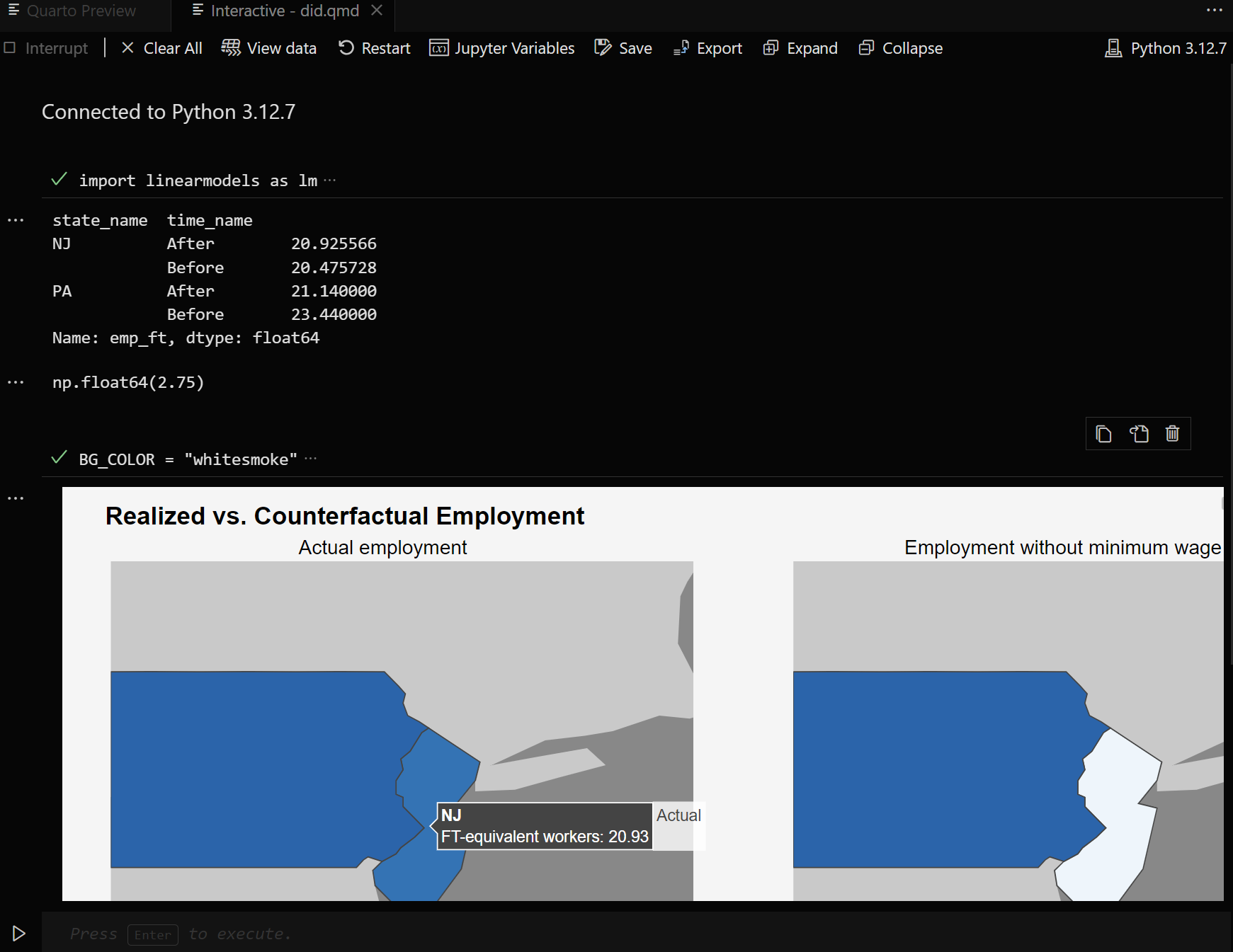
<p><img src="/assets/img/blog/blog-quarto-vs-view.png" alt="Quarto Slides in VS Code" /></p>

<p>This is exactly the workflow I had been looking for when embedding data or simulations into the presentation. If the code or data changes, I re-render and rerun everything. No exporting and re-importing (no awkward forgotten outdated figures!) unless I explicitly want to use specific fixed results.</p>

<p>Quarto also offers an interactive mode in VSCode. I can work with code chunks just like in a Jupyter Notebook, all within the same window and with the same source file. Once I’m happy with the results, I simply render the slide with the finalized code cells.</p>

<p><img src="/assets/img/blog/blog-quarto-vs-interactive.png" alt="Quarto Interactive Mode" /></p>

<h3 id="clean-syntax-maintainable-documents-straightforward-math">Clean Syntax, Maintainable Documents, Straightforward Math</h3>

<p>Quarto uses Markdown + code chunks. Slides are readable, easy to edit, and easy to return to later. This simplicity has made a big difference in my teaching and research prep. I spend less time fiddling  and more time refining the actual content. It’s also made it easier to reuse, adapt, and scale up materials across contexts.</p>

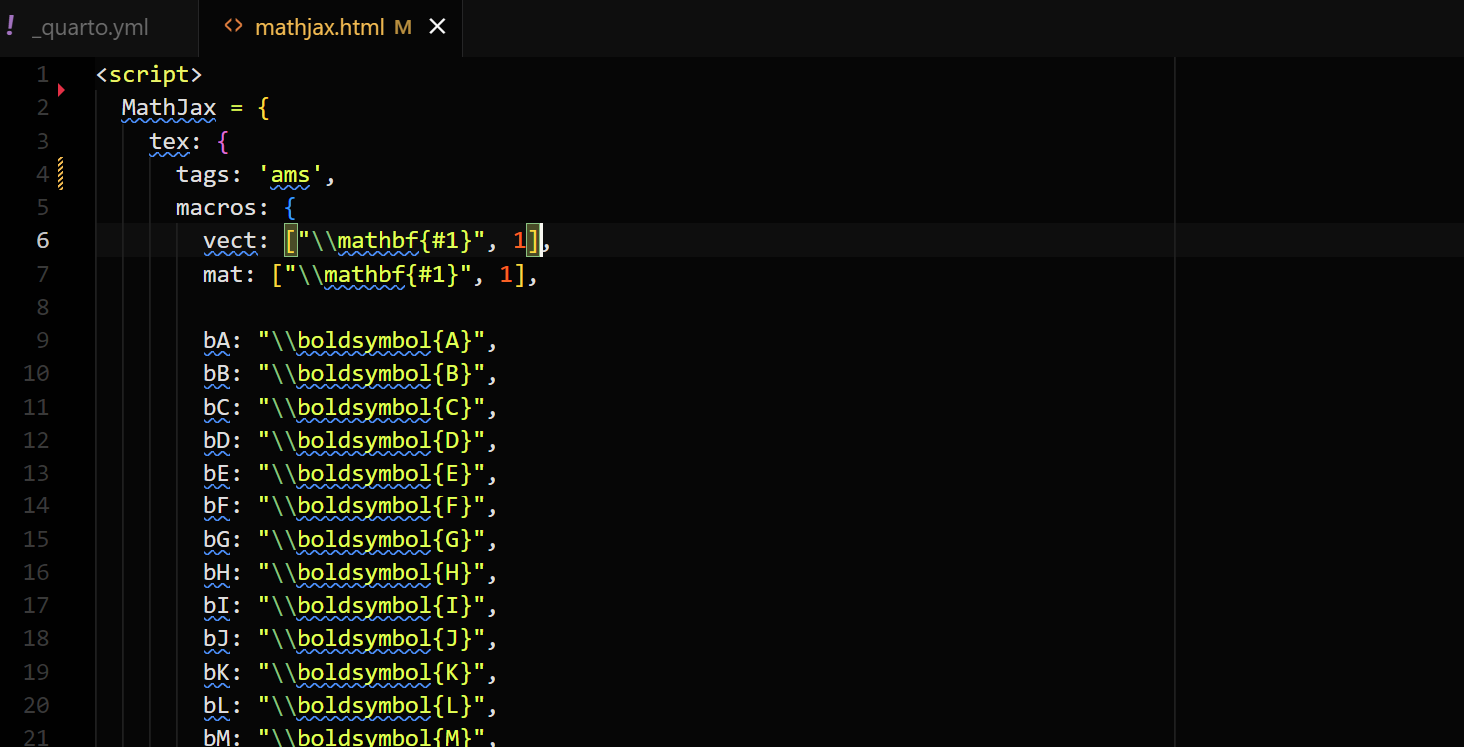
<p>Math support is also smooth. I have quite a few custom math macros. With HTML outputs, I can select MathJax as the math renderer, and I can define all my custom commands in a small <code class="language-plaintext highlighter-rouge">mathjax.html</code> file. Including that file in the header takes a single line in the YAML front matter, and the macros are then available throughout.</p>

<p><img src="/assets/img/blog/blog-quarto-vs-mathjax.png" alt="MathJax config file" /></p>

<h3 id="modern-output-responsive-customizable-cross-device">Modern Output: Responsive, Customizable, Cross-Device</h3>

<p>I now render slides to HTML using Reveal.js and present directly from the browser. That alone solves several longstanding problems:</p>

<ul>
  <li>Responsive layout: slides adapt well to different devices and projectors (no more misjudged aspect ratios).</li>
  <li>Easy customization: styling via themes or CSS is straightforward.</li>
  <li>Interactivity: I can embed Plotly plots or add tabs, collapsible code blocks, and other UI features with minimal effort.</li>
  <li>Portability: no need to worry about fonts, encoding, or PDF viewers. As long as there is an internet connection, all is good.</li>
</ul>

<p>I still generate PDFs for compatibility or archiving, but HTML is now my default. And if needed, the PDF can be generated straight from the browser version.</p>

<h3 id="stability-ie-less-fighting-with-my-tools">Stability (i.e. Less Fighting With My Tools)</h3>

<p>Perhaps most importantly: it’s stable.</p>

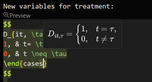
<p>I no longer have misleading errors and warnings in my life. Editor support (in VSCode) is excellent — I get previews, hover-rendered equations, linting, and clear error messages.</p>

<p><img src="/assets/img/blog/blog-quarto-vs-preview.png" alt="VSCode Equation Preview" /></p>

<p>This has quietly saved me a lot of frustration.</p>

<h3 id="a-portable-git-friendly-workflow">A Portable, Git-Friendly Workflow</h3>

<p>One of the biggest improvements: all my slides now live in Git repositories, are synced via GitHub, and deployed directly to my website. With Git, I can version-control my work and use issues and branches to organize myself. This aligns closely with the workflow I try to have: reproducibility, automation, and versioning are central.</p>

<h3 id="optional-interactivity">Optional Interactivity</h3>

<p>I don’t go overboard here, but having the option to include interactive elements is genuinely useful.</p>

<ul>
  <li>Live plots with Plotly.</li>
  <li>Hoverable explanations, collapsible blocks.</li>
  <li>Tabs for comparing different views or results.</li>
</ul>

<p>I think these things make the slides look better and add an extra layer of flexibility to visualizations.</p>

<h2 id="add-ons-that-i-like">Add-ons That I like</h2>

<p>There were only two things that I missed about Beamer — section header (in the spirit of the Berlin Beamer theme) and native TiKZ.</p>

<p>But even those things I was able to easily replicate with a couple of add-ons:</p>

<ul>
  <li><a href="https://github.com/shafayetShafee/reveal-header"><code class="language-plaintext highlighter-rouge">reveal-header</code></a>: lets you add a consistent header or logo to every slide.</li>
  <li><a href="https://github.com/pandoc-ext/diagram"><code class="language-plaintext highlighter-rouge">diagram</code></a>: supports embedded diagrams using Mermaid, GraphViz, TikZ, and others. I use it mostly for quick schema and causal graphs.</li>
</ul>

<h2 id="in-short">In Short</h2>

<p>Quarto has made my slides:</p>

<ul>
  <li>More reproducible</li>
  <li>Easier to maintain</li>
  <li>More portable and future-proof</li>
</ul>

<p>Beamer served its purpose for me. I appreciate what it made possible (and I think I’ve made some good-looking slides with it from time to time). But for the kind of work I do now, across teaching, research, and data science, Quarto has been a vastly better fit.</p>]]></content><author><name>Vladislav Morozov</name><email>vladislav.morozov [at] barcelonagse.eu</email></author><category term="Web" /><category term="Quarto" /><category term="Quarto" /><category term="Web" /><category term="Visualizations" /><summary type="html"><![CDATA[Why I switched from Beamer to Quarto Reveal.js for reproducible, maintainable, and portable slides in teaching, research, and data science.]]></summary><media:thumbnail xmlns:media="http://search.yahoo.com/mrss/" url="https://vladislav-morozov.eu/assets/img/blog/blog-quarto-example.gif" /><media:content medium="image" url="https://vladislav-morozov.eu/assets/img/blog/blog-quarto-example.gif" xmlns:media="http://search.yahoo.com/mrss/" /></entry><entry><title type="html">Visualizing Convergence in Probability and the Law of Large Numbers</title><link href="https://vladislav-morozov.eu/blog/statistics/theory/2025-04-21-visualizing-law-large-numbers-convergence-probability/" rel="alternate" type="text/html" title="Visualizing Convergence in Probability and the Law of Large Numbers" /><published>2025-04-21T00:00:00+00:00</published><updated>2025-04-21T00:00:00+00:00</updated><id>https://vladislav-morozov.eu/blog/statistics/theory/visualizing-law-large-numbers-convergence-probability</id><content type="html" xml:base="https://vladislav-morozov.eu/blog/statistics/theory/2025-04-21-visualizing-law-large-numbers-convergence-probability/"><![CDATA[<script type="text/x-mathjax-config">
MathJax.Hub.Config({
 "HTML-CSS": { linebreaks: { automatic: true } },
         SVG: { linebreaks: { automatic: true } }
});
</script>

<script type="text/javascript">
if (window.MathJax) {
  MathJax.Hub.Queue(
    ["Typeset",MathJax.Hub]
  );
}
</script>

<p>Convergence in probability is fundamental to statistical inference. It underpins most large-sample approximations, while consistency is a basic requirement for any sensible estimator. While the formal definition is simple, building an intuitive understanding is a bit challenging. This post explores two “honest” ways to visualize convergence in probability, using the law of large numbers as an example.</p>

<!--more-->

<ul id="markdown-toc">
  <li><a href="#reminder-convergence-in-probability-and-the-weak-law-of-large-numbers" id="markdown-toc-reminder-convergence-in-probability-and-the-weak-law-of-large-numbers">Reminder: Convergence in Probability and the Weak Law of Large Numbers</a></li>
  <li><a href="#the-usual-ways" id="markdown-toc-the-usual-ways">The “Usual” Ways</a></li>
  <li><a href="#two-better-ways" id="markdown-toc-two-better-ways">Two Better Ways</a>    <ul>
      <li><a href="#direct-visualization-of-probabilities-right-panel" id="markdown-toc-direct-visualization-of-probabilities-right-panel">Direct Visualization of Probabilities (Right Panel)</a></li>
      <li><a href="#cdf-convergence-left-panel" id="markdown-toc-cdf-convergence-left-panel">CDF convergence (left panel)</a></li>
    </ul>
  </li>
</ul>

<p class="note" title="Attention">If math is messed up, <span style="color:red">reload</span> the page so that MathJax has another go.</p>

<h2 id="reminder-convergence-in-probability-and-the-weak-law-of-large-numbers">Reminder: Convergence in Probability and the Weak Law of Large Numbers</h2>

<p>To start, recall that a sequence \(X_1, X_2, \dots\) converges in probability to \(X\) if for every \(\varepsilon&gt;0\) the probability of \(X_n\) deviating from \(X\) by more than \(\varepsilon\) tends to zero as \(n\to\infty\)</p>

\[P(|X_n-X|&gt;\varepsilon) \to 0\]

<p>The simplest weak law of large numbers simply says the following. If \(X_1, X_2, ...\) are independently and identically distributed with a finite mean \(\mathbb{E}[X_i]\), then the average of these variables converges to \(\mathbb{E}[X_i]\) precisely in the above sense: for any \(\varepsilon&gt;0\) it holds that</p>

\[P(|\bar{X}-\mathbb{E}[X_i]|&gt;\varepsilon) \to 0\]

<h2 id="the-usual-ways">The “Usual” Ways</h2>

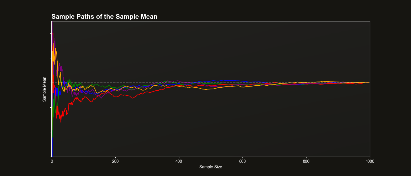
<p>A common way to visualize the law of large numbers is to plot the path of the sample mean as the sample size increases. For example:</p>

<p><img src="/assets/img/blog/blog-lln-sample-paths.png" alt="Example sample mean sample path plot" /></p>

<p>The plot above shows several trajectories of the sample mean across increasing sample sizes. The horizontal dashed line represents the true population mean.</p>

<p>While this visualization has some appeal, it actually at best illustrates almost sure convergence. Almost sure convergence is a stronger and more technical concept that usually only makes sense after some real analysis, but not in a first course in probability or statistics. More importantly, the above plot doesn’t connect visually to the definition involving probabilities.</p>

<h2 id="two-better-ways">Two Better Ways</h2>

<p>Unfortunately, there is no way around it — convergence in probability has to do with convergence of, well, probabilities. The best approach is then to honestly visualize such probabilities.</p>

<p>Here are two proposals, shown in the animated plot on top of the page.</p>

<h3 id="direct-visualization-of-probabilities-right-panel">Direct Visualization of Probabilities (Right Panel)</h3>

<p>Choose a few values of \(\varepsilon\) and plot the probability that the
sample mean deviates from the population mean by more than \(\varepsilon\)
as a function of sample size. This aligns exactly with the definition of
convergence in probability and shows how these deviation probabilities
shrink.</p>

<h3 id="cdf-convergence-left-panel">CDF convergence (left panel)</h3>

<p>Plot the empirical cumulative distribution function (CDF) of the sample
mean. As the sample size increases, this CDF collapses to the CDF of the
constant \(\mathbb{E}[X_i]\) — 0 below that value, 1 starting from
\(\mathbb{E}[X_i]\). This shows convergence in distribution, which (when
the limit is a constant) is equivalent to convergence in probability. A nice feature is that this approach visualizes all the probabilities at the same time.</p>

<p>This second method also improves on another common visualization:
plotting histograms or densities of the sample mean across replications.
While intuitive, convergence of histograms/densities is actually
convergence in total variation, a much stronger notion that’s not quite relevant here. Using the CDF instead keeps the focus on the core idea.</p>]]></content><author><name>Vladislav Morozov</name><email>vladislav.morozov [at] barcelonagse.eu</email></author><category term="Statistics" /><category term="Theory" /><category term="Asymptotics" /><summary type="html"><![CDATA[How to visualize convergence in probability and the weak law of large numbers directly and honestly]]></summary><media:thumbnail xmlns:media="http://search.yahoo.com/mrss/" url="https://vladislav-morozov.eu/assets/img/blog/blog-lln.gif" /><media:content medium="image" url="https://vladislav-morozov.eu/assets/img/blog/blog-lln.gif" xmlns:media="http://search.yahoo.com/mrss/" /></entry><entry><title type="html">Why Simultaneous (Joint) Tests Instead of Adjusted Multiple Tests?</title><link href="https://vladislav-morozov.eu/blog/statistics/inference/2025-04-01-why-joint-test/" rel="alternate" type="text/html" title="Why Simultaneous (Joint) Tests Instead of Adjusted Multiple Tests?" /><published>2025-04-01T00:00:00+00:00</published><updated>2025-04-01T00:00:00+00:00</updated><id>https://vladislav-morozov.eu/blog/statistics/inference/why-joint-test</id><content type="html" xml:base="https://vladislav-morozov.eu/blog/statistics/inference/2025-04-01-why-joint-test/"><![CDATA[<script type="text/x-mathjax-config">
MathJax.Hub.Config({
 "HTML-CSS": { linebreaks: { automatic: true } },
         SVG: { linebreaks: { automatic: true } }
});
</script>

<script type="text/javascript">
if (window.MathJax) {
  MathJax.Hub.Queue(
    ["Typeset",MathJax.Hub]
  );
}
</script>

<p>When testing multiple hypotheses in a regression, why do we use simultaneous (joint) tests instead of just adjusting the \(p\)-values from separate \(t\)-tests? The usual answer is a vague statement that simultaneous tests are more powerful. This post quantifies that statement and also finds that the story is more nuanced than that.</p>

<!--more-->

<!-- - [Introduction](#introduction)
- [Some Theory: Simultaneous vs. Multiple
  Testing](#some-theory-simultaneous-vs-multiple-testing)
  - [Simultaneous Tests](#simultaneous-tests)
  - [Multiple Tests](#multiple-tests)
- [So Why Simultaneous Testing?](#so-why-simultaneous-testing)
  - [Simulation Settings](#simulation-settings)
  - [Results](#results)
  - [Why the Disparity in Power?](#why-the-disparity-in-power)
- [Conclusion](#conclusion) -->

<ul id="markdown-toc">
  <li><a href="#introduction" id="markdown-toc-introduction">Introduction</a></li>
  <li><a href="#some-theory-simultaneous-vsmultiple-testing" id="markdown-toc-some-theory-simultaneous-vsmultiple-testing">Some Theory: Simultaneous vs. Multiple Testing</a>    <ul>
      <li><a href="#simultaneous-tests" id="markdown-toc-simultaneous-tests">Simultaneous Tests</a></li>
      <li><a href="#multiple-tests" id="markdown-toc-multiple-tests">Multiple Tests</a>        <ul>
          <li><a href="#combining-multiple-t-tests" id="markdown-toc-combining-multiple-t-tests">Combining Multiple \(t\)-Tests</a></li>
          <li><a href="#critical-values-and-the-multiple-choice-problem" id="markdown-toc-critical-values-and-the-multiple-choice-problem">Critical Values and the Multiple Choice Problem</a></li>
          <li><a href="#bonferroni-correction" id="markdown-toc-bonferroni-correction">Bonferroni Correction</a></li>
        </ul>
      </li>
    </ul>
  </li>
  <li><a href="#so-why-simultaneous-testing" id="markdown-toc-so-why-simultaneous-testing">So Why Simultaneous Testing?</a>    <ul>
      <li><a href="#simulation-settings" id="markdown-toc-simulation-settings">Simulation Settings</a></li>
      <li><a href="#results" id="markdown-toc-results">Results</a></li>
      <li><a href="#why-the-disparity-in-power" id="markdown-toc-why-the-disparity-in-power">Why the Disparity in Power?</a></li>
    </ul>
  </li>
  <li><a href="#conclusion" id="markdown-toc-conclusion">Conclusion</a></li>
</ul>

<p class="note" title="Attention">If math is messed up, <span style="color:red">reload</span> the page so that MathJax has another go.</p>

<h2 id="introduction">Introduction</h2>

<p>When teaching undergraduate econometrics, we eventually reach
multivariate regression. This is where hypothesis testing becomes more
complex — hypotheses may now involve multiple restrictions on several
coefficients at the same time. To handle this, we introduce \(F\) or Wald
tests, which evaluate hypotheses simultaneously (“jointly”) using a
single statistic.</p>

<p>But is this the only way? At least in some years, the students were
already familiar with the multiple testing problem and Bonferroni
corrections. Naturally, the question always came up: why introduce a
whole new test when we could just combine several familiar \(t\)-tests,
adjusting the critical values for multiple comparisons.</p>

<p>My usual answer was that multiple testing adjustments ignore the
structure of the problem, making them potentially less powerful. But I
never had a concrete numerical example to illustrate this point.</p>

<p>So, I decided to take a closer look at a textbook case and run a
simulation. As it turns out, the usual answer is mostly right — but not
entirely. Adjusted multiple testing can indeed lead to a massive loss of
power compared to simultaneous testing. However, in some cases
(surprisingly!), simultaneous testing actually performs slightly worse.</p>

<h2 id="some-theory-simultaneous-vsmultiple-testing">Some Theory: Simultaneous vs. Multiple Testing</h2>

<p>Specifically, to construct the example and discuss the approaches, let’s
look at a simple regression model with a constant and two covariates:</p>

\[y_{i} = \alpha  + \beta_1 x_i^{(1)} + \beta_2 x_i^{(2)} + u_i,\]

<p>The null hypothesis of interest is</p>

\[H_0: \beta_1 = \beta_2 = 0.\]

<p>This \(H_0\) is “joint” because it involves multiple parameters at
once.</p>

<p>How do we test \(H_0\)? As I mentioned above, there are two approaches:</p>

<ol>
  <li>Simultaneously with a single statistic.</li>
  <li>By combining multiple tests.</li>
</ol>

<h3 id="simultaneous-tests">Simultaneous Tests</h3>

<p>As soon as the above \(H_0\) is first encountered, any econometrics
textbook will introduce the simultaneous testing approach. In
simultaneous testing, we create a single test statistic, like the Wald
statistic. The Wald test statistic \(\hat{W}\) for the above \(H_0\) is
constructed using the coefficient estimates and their estimated
variance-covariance matrix:</p>

\[\hat{W} = n\hat{\boldsymbol{\beta}}'(\widehat{\mathrm{Avar}}(\hat{\boldsymbol{\beta}}))^{-1}\hat{\boldsymbol{\beta}},\]

<p>where \(n\) is the sample size,
\(\hat{\boldsymbol{\beta}} = (\hat{\beta}_1, \hat{\beta}_2)\), and
\(\widehat{\mathrm{Avar}}(\hat{\boldsymbol{\beta}})\) is the estimated
asymptotic variance-covariance matrix of \(\hat{\boldsymbol{\beta}}\).</p>

<p>Under mild assumption, \(\hat{W}\) will converge in distribution to a
\(\chi^2_2\) random variable. A size \(\alpha\) Wald test rejects \(H_0\) is
\(\hat{W}\) exceeds the \((1-\alpha)\)th quantile of \(\chi^2_2\).</p>

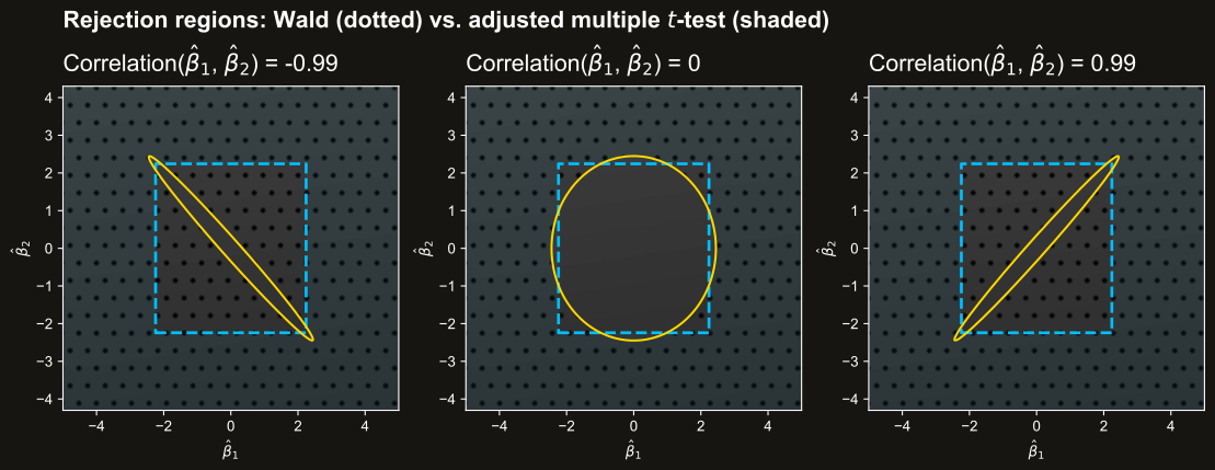
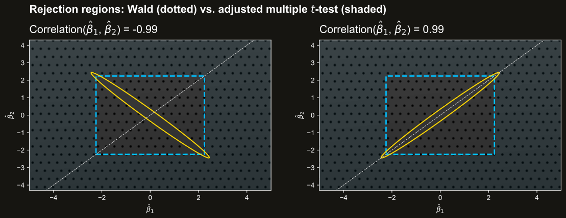
<p>For our simple case, you can draw the decision regions of the test
graphically in the space of estimates. The figure below shows the
rejection region for a few different values of the correlation between
\(\hat{\beta}_1\), \(\hat{\beta}_2\). If \((\hat{\beta}_1, \hat{\beta}_2)\)
fall outside the yellow ellipse into the dotted area, the test rejects
\(H_0\).</p>

<p><img src="/assets/img/blog/blog-simultaneous-tests-rejection_regions.svg" alt="Rejection regions for tests
compared" title="Rejection regions for the tests compared" /></p>

<h3 id="multiple-tests">Multiple Tests</h3>

<h4 id="combining-multiple-t-tests">Combining Multiple \(t\)-Tests</h4>

<p>Instead of testing both coefficients jointly, another approach is to
test them separately and adjust for multiple comparisons. How does this
work? The idea is simple: perform a \(t\)-test for each coefficient
individually. If either \(t\)-test rejects, reject the joint null
hypothesis.</p>

<p>Formally, we compute the \(t\)-statistics for the \(k\)th coefficient as</p>

\[t_k = \dfrac{\sqrt{n}\hat{\beta_k}}{\widehat{\mathrm{Avar}}(\hat{\beta}_k)}\]

<p>A test for our \(H_0\) rejects if
\(\max\lbrace |{t}_1|, |{t}_2| \rbrace\) exceeds some prespecified
critical value \(c_{\alpha}\).</p>

<h4 id="critical-values-and-the-multiple-choice-problem">Critical Values and the Multiple Choice Problem</h4>

<p>Key question: how do you set the critical value \(c_{\alpha}\) to ensure
that the test has the correct size \(\alpha\)? Let’s examine the rejection
probabilities under \(H_0\):</p>

\[\begin{aligned}
&amp; P(\text{test rejects}|H_0) \\
&amp; = P(\max\lbrace |{t}_1|, |{t}_2| \rbrace \geq c_{\alpha}|H_0) \\
&amp; = P\left( \lbrace |{t}_1| \geq c_{\alpha}\rbrace \cup \lbrace |{t}_2| \geq c_{\alpha}\rbrace |H_0 \right) \\
&amp; = P\left( \lbrace |{t}_1| \geq c_{\alpha}\rbrace   |H_0 \right) + P\left(   \lbrace |{t}_2| \geq c_{\alpha}\rbrace |H_0 \right)  \\
&amp; \quad - P\left( \lbrace |{t}_1| \geq c_{\alpha}\rbrace \cap \lbrace |{t}_2| \geq c_{\alpha}\rbrace |H_0 \right),
\end{aligned}\]

<p>where we have used the inclusion-exclusion principle in the last
line.</p>

<p>We can’t use the typical critical values from individual \(t\)-tests
(i.e., the \((1-\alpha/2)\)th quantile of the \(N(0, 1)\) distribution). To
see why, note that with this choice
\(P\left( \lbrace |{t}_1| \geq c_{\alpha}\rbrace   |H_0 \right) = \alpha\)
(at least asymptotically). Meanwhile, the probability of the
intersection lies somewhere between \(0\) and \(\alpha\), depending on the
dependence between the test statistics. We can then conclude that</p>

\[P(\text{test rejects}|H_0) \in [\alpha, 2\alpha].\]

<p>In words, if you do the individual \(t\)-tests with size \(\alpha\), the
combination can actually have size \(2\alpha\) (e.g., 10%, if using 5%
critical values). We will be rejecting the null too often even if it is
true. Intuitively, there are more opportunities for large enough
estimation error to slip through — see this excellent <a href="https://xkcd.com/882/">xkcd
strip</a>.</p>

<p>The above issue is known as the multiple testing problem. For a deeper
dive into the multiple testing problem, check out chapter 9 in the
excellent book by Lehmann and Romano (2022).</p>

<h4 id="bonferroni-correction">Bonferroni Correction</h4>

<p>A simple solution to the problem is to simply adjust critical values in
the individual component tests. If we take size-\((\alpha/2)\) critical
values, the above test will reject with frequency \(\leq \alpha\) under
the null — exactly what we want. That’s the idea of the Bonferroni
correction, the simplest possible approach, though not the only one. In
our case, if we want a test with level at most 5%, we will do the
individual \(t\)-tests with values for \(2.5%\) (that is, the \(0.9875\)th
quantile of the normal distribution).</p>

<h2 id="so-why-simultaneous-testing">So Why Simultaneous Testing?</h2>

<p>Given that both approaches control size correctly, why do we typically
prefer simultaneous tests? It’s not because they are easier to compute —
simultaneous tests often require more statistical infrastructure.
Instead, the key reason is power.</p>

<p>Recall that power, in simple terms, is the ability of a test to detect
true effects. More powerful tests are more likely to reject \(H_0\) when
the true parameters lie outside it — meaning they can detect real
effects with higher probability.</p>

<p>It makes sense that simultaneous testing would be more powerful. If we
look back at the rejection region image, we see that the Wald test
adjusts for the dependence between \(\hat{\beta}_1\) and \(\hat{\beta}_2\),
while the multiple \(t\)-test combination doesn’t. In other words, the
Wald test makes better use of the available information than multiple
testing adjustments.</p>

<h3 id="simulation-settings">Simulation Settings</h3>

<p>However, intuition can be wrong and needs to be checked one way or
another. To check whether it holds, let’s take a look at a simple
simulation for the above model. We’ll draw \((x_{i}^{(1)}, x_{i}^{(2)})\)
and \(u_{i}\) from suitable normal distributions:</p>

\[\begin{aligned}
u_{i} &amp; \sim N(0, 1), \\
\begin{pmatrix}
x_i^{(1)} \\
x_i^{(2)}
\end{pmatrix} &amp; \sim N\left(\begin{pmatrix}
1 \\
1
\end{pmatrix}, \begin{pmatrix}
1 &amp; \rho \\
\rho &amp; 1
\end{pmatrix} \right)
\end{aligned},\]

<p>where the correlation \(\rho\) will run between \(-1\) and \(1\). This nice
normal setup reflects the canonical case first discussed in textbooks.
You can also view it as an asymptotic approximation to a more general
data-generating process.</p>

<p>To be able to visualize the results, I set \(\beta_1 = \beta_2 =c\), and
then vary the common coefficient value \(c\). This setup might seem
restrictive, but the results are actually quite general. By
appropriately rescaling \((x_{i}^{(1)}, x_{i}^{(2)})\), any other
configuration of \((\beta_1, \beta_2)\) can be reduced to a case with
\(\beta_1=\beta_2\).</p>

<p>In this context, we can compute the power of the simultaneous Wald test
and the power of adjusted multiple \(t\)-test. I’ll use the Bonferroni
adjustment, and also the slightly more sophisticated Holm-Šidák method.</p>

<p>The full Python code for the simulations can be found in the blog GitHub
repo.</p>

<p align="center">

<a href="https://github.com/vladislav-morozov/blog-code-hub"><img src="https://gh-card.dev/repos/vladislav-morozov/blog-code-hub.svg" /></a>
</p>

<h3 id="results">Results</h3>

<p>Now, let’s compare the power of simultaneous and multiple tests across
different values of \(c\) and the correlation between \(\hat{\beta}_1\) and
\(\hat{\beta}_2\) (approximately \(-\rho\)) The figure below depicts the
difference in power between the Wald test and the two difference
adjustments for the multiple \(t\)-tests, all as a function of \(c\) and the
correlation between \(\hat{\beta}_1\) and \(\hat{\beta}_2\) (equal to
approximately \(-\rho\)).</p>

<p><img src="/assets/img/blog/blog-simultaneous-tests-power-results.svg" alt="Differences in power between a simultaneous Wald test and multiple
adjusted
$$t$$-tests" title="Differences in power between a simultaneous Wald test and multiple adjusted $$t$$-tests" /></p>

<p>The differences in power are striking when the coefficient estimators
are negatively correlated. In some cases, the Wald test almost always
rejects \(H_0\), while the multiple \(t\)-test barely does.</p>

<p>To check that the above results are not due to something crazy in the
test behavior, we also need to take a look at the actual power surfaces.
The image below plots them on the same axes as above. See the animated
plot on top of the page for a view of all the power plots for individual
values of the correlation between \(\hat{\beta}_1\) and \(\hat{\beta}_2\).</p>

<p><img src="/assets/img/blog/blog-simultaneous-tests-power-surfaces.svg" alt="Power of simultaneous Wald test and multiple adjusted
$$t$$-tests" title="Power of simultaneous Wald test and multiple adjusted $$t$$-tests" /></p>

<p>Overall, it seems that both kinds of tests behave sensibly by
themselves.</p>

<p>With the above plots in hand, I’d like to highlight three points of
contrast between the tests:</p>

<ol>
  <li>
    <p>Simultaneous tests can be dramatically more powerful than multiple
tests when \(\hat{\beta}_1\) and \(\hat{\beta}_2\) are negatively
correlated, especially for moderate deviations from \(H_0\).</p>
  </li>
  <li>
    <p>This advantage fades as the correlation weakens — when
\(\hat{\beta}_1\) and \(\hat{\beta}_2\) are uncorrelated, the two
methods perform similarly.</p>
  </li>
  <li>
    <p>For positive correlation, the Wald test actually loses some power,
but the gap is much smaller than in the negative case.</p>
  </li>
</ol>

<p>In short, our intuition is only mostly right. Simultaneous tests do not
always dominate multiple adjusted tests in terms of power. However, when
simultaneous tests are better, they are so by such a huge margin that it
is hard to imagine a situation where one would prefer the multiple
testing approach.</p>

<h3 id="why-the-disparity-in-power">Why the Disparity in Power?</h3>

<p>Why does this power difference occur? And why is it more pronounced for
negative correlation?</p>

<p>As it turns out, the case of negative and positive correlation are
actually asymmetric in terms of test behavior. The image below slices
out the power curves for two extreme cases:</p>

<p><img src="/assets/img/blog/blog-simultaneous-tests-power-slices.svg" alt="Power of simultaneous Wald test and multiple adjusted
$$t$$-tests" title="Power of simultaneous Wald test and multiple adjusted $$t$$-tests" /></p>

<p>The multiple \(t\)-test performs similarly in both cases. However, the
Wald test is much better in the negatively correlated case than in the
positively correlated one.</p>

<p>Why? This result has to do with the shape of the rejection regions and
with how the coefficient estimators behave in this case. Let’s plot
those regions again, this time with the line \(\beta_1=\beta_2=c\) on
which the true coefficients lie: <img src="/assets/img/blog/blog-simultaneous-tests-rejection_regions-line.svg" alt="Rejection regions for tests
compared" title="Rejection regions for tests compared" /></p>

<p>The short story is that the power profile is determined by how much the
rejection regions cover of the line \(\beta_1=\beta_2\). More of the line
covered \(=\) higher power. The long story is as follows:</p>

<ul>
  <li>
    <p>When \(\hat{\beta}_1\) and \(\hat{\beta}_2\) are negatively correlated,
estimation errors tend to push them in opposite directions from the
line \(\beta_1=\beta_2\). Under the null, these errors are likely to
fall on the line \(\beta_2=-\beta_1\). The Wald test positions its
rejection region accordingly and excludes a section from that line. As
a result, the rejection region fails to cover only a small section of
the \(\beta_1=\beta_2\) line.</p>
  </li>
  <li>
    <p>In contrast, for positive correlation, estimation errors tend to move
together along the \(\beta_1 = \beta_2\) line. To guarantee correct
size, the Wald test has to exclude more of the line than the multiple
\(t\)-tests from the rejection regions.</p>
  </li>
</ul>

<p>Finally, I want to again point out that the results are somewhat more
general than they look. By suitably rescaling the covariates, one can
always rescale the coefficients so that they are equal. Then the above
discussion would apply in full.</p>

<h2 id="conclusion">Conclusion</h2>

<p>In conclusion, the usual vague explanation that simultaneous tests are
more powerful turns out to be mostly — but not always — true. While
simultaneous testing does not uniformly outperform multiple testing,
when it does, the improvement is substantial. Given this, it’s hard to
justify using multiple testing adjustments over simultaneous tests in
most practical situations. I think explaining this point with hard
evidence may help people understand why we introduce and do simultaneous
tests.</p>

<div id="refs" class="references csl-bib-body hanging-indent" entry-spacing="0">

<div id="ref-Lehmann2022TestingStatisticalHypotheses" class="csl-entry">

Lehmann, Erich L., and Joseph P. Romano. 2022. Testing Statistical
Hypotheses. 4th ed. Springer Cham.
&lt;https://doi.org/10.1007/978-3-030-70578-7&gt;.

</div>

</div>]]></content><author><name>Vladislav Morozov</name><email>vladislav.morozov [at] barcelonagse.eu</email></author><category term="Statistics" /><category term="Inference" /><category term="Python" /><category term="Simulations" /><category term="Inference" /><summary type="html"><![CDATA[Why simultaneous hypothesis tests are better — but not always — than adjusted multiple tests]]></summary><media:thumbnail xmlns:media="http://search.yahoo.com/mrss/" url="https://vladislav-morozov.eu/assets/img/blog/blog-why-joint-testing-animated.gif" /><media:content medium="image" url="https://vladislav-morozov.eu/assets/img/blog/blog-why-joint-testing-animated.gif" xmlns:media="http://search.yahoo.com/mrss/" /></entry><entry><title type="html">Why Adding Fixed Effects May Increase Bias</title><link href="https://vladislav-morozov.eu/blog/statistics/heterogeneity/2025-02-01-fixed_effects_danger/" rel="alternate" type="text/html" title="Why Adding Fixed Effects May Increase Bias" /><published>2025-02-01T00:00:00+00:00</published><updated>2025-02-01T00:00:00+00:00</updated><id>https://vladislav-morozov.eu/blog/statistics/heterogeneity/fixed_effects_danger</id><content type="html" xml:base="https://vladislav-morozov.eu/blog/statistics/heterogeneity/2025-02-01-fixed_effects_danger/"><![CDATA[<script type="text/x-mathjax-config">
MathJax.Hub.Config({
 "HTML-CSS": { linebreaks: { automatic: true } },
         SVG: { linebreaks: { automatic: true } }
});
</script>

<script type="text/javascript">
if (window.MathJax) {
  MathJax.Hub.Queue(
    ["Typeset",MathJax.Hub]
  );
}
</script>

<p>A common approach to controlling for unobserved heterogeneity is to run a linear regression with fixed effects. This post shows that this strategy may lead to strong bias in more realistic settings, even if you specify the fixed effects correctly. It is also about some things you can do about it.</p>

<!--more-->

<!-- ## Contents -->
<!-- 
- [Introduction](#introduction-the-problem)
  - [The Setting](#the-setting)
  - [The Problem with Fixed Effects and This
    Post](#the-problem-with-fixed-effects-and-this-post)
- [A Simulation Study: the Issues of the FE
  Estimator](#a-simulation-study-the-issues-of-the-fe-estimator)
- [When the FE Estimators Is Usable (and When
  Not)](#when-the-fe-estimators-is-usable-and-when-not)
- [Practical Advice and Conclusions](#practical-advice-and-conclusions) -->

<ul id="markdown-toc">
  <li><a href="#introduction-the-problem" id="markdown-toc-introduction-the-problem">Introduction: the Problem</a>    <ul>
      <li><a href="#the-setting" id="markdown-toc-the-setting">The Setting</a></li>
      <li><a href="#the-problem-with-fixed-effects-and-this-post" id="markdown-toc-the-problem-with-fixed-effects-and-this-post">The Problem with Fixed Effects and This Post</a></li>
    </ul>
  </li>
  <li><a href="#a-simulation-study-the-issues-of-the-fe-estimator" id="markdown-toc-a-simulation-study-the-issues-of-the-fe-estimator">A Simulation Study: the Issues of the FE Estimator</a>    <ul>
      <li><a href="#setting-and-estimators-compared" id="markdown-toc-setting-and-estimators-compared">Setting and Estimators Compared</a></li>
      <li><a href="#results-distribution-of-estimators" id="markdown-toc-results-distribution-of-estimators">Results: Distribution of Estimators</a></li>
      <li><a href="#takeaway-do-not-trust-estimate-changes-after-adding-fixed-effects" id="markdown-toc-takeaway-do-not-trust-estimate-changes-after-adding-fixed-effects">Takeaway: Do Not Trust Estimate Changes after Adding Fixed Effects</a></li>
    </ul>
  </li>
  <li><a href="#when-the-fe-estimators-is-usable-and-when-not" id="markdown-toc-when-the-fe-estimators-is-usable-and-when-not">When the FE Estimators Is Usable (and When Not)</a>    <ul>
      <li><a href="#conditions-for-consistency-of-the-fe-estimator" id="markdown-toc-conditions-for-consistency-of-the-fe-estimator">Conditions for Consistency of the FE Estimator</a></li>
      <li><a href="#a-sufficient-condition-for-mathbbetildeboldsymbolx_itildeboldsymbolx_iboldsymboleta_i0" id="markdown-toc-a-sufficient-condition-for-mathbbetildeboldsymbolx_itildeboldsymbolx_iboldsymboleta_i0">A Sufficient Condition for \(\mathbb{E}[\tilde{\boldsymbol{X}}_i'\tilde{\boldsymbol{X}}_i\boldsymbol{\eta}_i]=0\)</a></li>
      <li><a href="#mathbbetildeboldsymbolx_itildeboldsymbolx_iboldsymboleta_i-and-adding-more-effects" id="markdown-toc-mathbbetildeboldsymbolx_itildeboldsymbolx_iboldsymboleta_i-and-adding-more-effects">\(\mathbb{E}[\tilde{\boldsymbol{X}}_i'\tilde{\boldsymbol{X}}_i\boldsymbol{\eta}_i]\) and Adding More Effects</a></li>
    </ul>
  </li>
  <li><a href="#practical-advice-and-conclusions" id="markdown-toc-practical-advice-and-conclusions">Practical Advice and Conclusions</a>    <ul>
      <li><a href="#solution-1-an-honest-approach-to-the-fe-estimator" id="markdown-toc-solution-1-an-honest-approach-to-the-fe-estimator">Solution 1: An Honest Approach to the FE Estimator</a></li>
      <li><a href="#solution-2-a-robust-approach-with-the-mean-group-estimator" id="markdown-toc-solution-2-a-robust-approach-with-the-mean-group-estimator">Solution 2: A Robust Approach with the Mean Group Estimator</a></li>
      <li><a href="#solution-3-a-robust-approach-with-grouped-estimation" id="markdown-toc-solution-3-a-robust-approach-with-grouped-estimation">Solution 3: A Robust Approach with Grouped Estimation</a></li>
      <li><a href="#conclusions" id="markdown-toc-conclusions">Conclusions</a></li>
    </ul>
  </li>
  <li><a href="#references" id="markdown-toc-references">References</a></li>
</ul>

<p class="note" title="Attention">If math is messed up, <span style="color:red">reload</span> the page so that MathJax has another go.</p>

<h2 id="introduction-the-problem">Introduction: the Problem</h2>

<h3 id="the-setting">The Setting</h3>

<p>Suppose that we want to estimate the average effect of some variables
\(\boldsymbol{x}\) on some outcome \(y\). For example, \(\boldsymbol{x}\) can
be investment in R&amp;D by a firm, and \(y\) can be worker productivity. In
another example, \(\boldsymbol{x}\) can be air pollution on a given day,
and \(y\) can be the crime rate on that day.</p>

<p>By now everyone agrees that you have to do something about <em>unobserved
heterogeneity</em> — there is a lot of unobserved differences between units
in any economic and business data. Firms differ in their technology,
culture, and managerial capacity, etc. Consumers differ in their
preferences, social ties, and expectations; etc.</p>

<p><strong>Common approach: adding fixed effects</strong> A common solution is to obtain
panel data and run a linear regression with “fixed effects”
(FEs):</p>

<p><span id="eq-homogeneous">
\(\hspace{1cm} y_{it} = \alpha_i +  (\text{other fixed effects}_{it}) + \boldsymbol{\beta}' \boldsymbol{x}_{it} + u_{it}, \quad i=1,\dots, N, \quad t=1, \dots, T \qquad (1)\)
 </span></p>

<p>The fixed effects are just heterogeneous constants.
The simplest kind are the unit-level effects \(\alpha_i\). Other effects
can include time-specific intercepts \(\delta_t\) (two-way FEs), or some
more complex combinations, such as industry \(\times\) year interacted
FEs.</p>

<p>The hope is that you will “control” for unobserved heterogeneity if you add “enough” FEs. In this case,  \(\boldsymbol{\beta}\) should capture the
effect of \(\boldsymbol{x}\) on \(y\). \(\boldsymbol{\beta}\) can be estimated
by eliminating the FEs from
<a href="#eq-homogeneous" class="quarto-xref">Equation 1</a> and
estimating the resulting equation — an approach known as <em>FE</em> (or
<em>within</em>) estimation.</p>

<h3 id="the-problem-with-fixed-effects-and-this-post">The Problem with Fixed Effects and This Post</h3>

<p><strong>But why homogeneous \(\boldsymbol{\beta}\)?</strong> A key problem with
<a href="#eq-homogeneous" class="quarto-xref">Equation 1</a> is that it
is not an internally consistent model. Why should the slopes
\(\boldsymbol{\beta}\) be the same for all units? This assumption goes
against acknowledging heterogeneity and including FEs. Would it not be
reasonable to specify the more flexible model where the slopes can also
be heterogeneous:</p>

<p><span id="eq-heterogenous">\(\hspace{1cm} y_{it} = \alpha_i +  (\text{other fixed effects}_{it}) + \color{red}{\boldsymbol{\beta}_i}' \boldsymbol{x}_{it} + u_{it}, \quad i=1,\dots, N, \quad t=1, \dots, T
 \qquad(2)\)</span></p>

<p>I personally struggle to think of a single convincing example where the
\(\boldsymbol{\beta}\) are homogeneous, while the constant terms can be
heterogeneous.</p>

<p><strong>What is this post about? Problems with FEs and Solutions</strong> In this
post, I show that the strategy of using FEs breaks down under the more
realistic <a href="#eq-heterogenous" class="quarto-xref">Equation 2</a>
and discuss some solutions. Specifically, we will see that:</p>

<ol>
  <li>
    <p>The FE estimator may be catastrophically biased even if you
correctly specify the FEs.</p>
  </li>
  <li>
    <p>If you add additional fixed effects, you may <em>increase</em> bias in
estimation and get worse results than if you didn’t do anything
about heterogeneity.</p>
  </li>
  <li>
    <p>There is a precise condition on the data under which the FE
estimator does correctly estimate the average effects.</p>
  </li>
  <li>
    <p>Some solutions are available: ranging from simply explicitly
thinking about the assumptions needed for consistent estimation to
using estimators robust to parameter heterogeneity.</p>
  </li>
</ol>

<p>The full simulation code is available on the blog codes
<a href="https://github.com/vladislav-morozov/blog-code-hub/tree/main/Statistics/Heterogeneity/fixed-effects-dangers">repository</a>.</p>

<p class="note" title="Remark">The issues with the fixed effects estimators are well-known
at least in the case of two-way effects in diff-in-diff settings (De
Chaisemartin and D’Haultfœuille 2020).
This post argues that the problems with FE estimators are much more
general: the appear in all contexts, no just diff-in-diff, and affect
any configuration of fixed effects.</p>

<h2 id="a-simulation-study-the-issues-of-the-fe-estimator">A Simulation Study: the Issues of the FE Estimator</h2>

<h3 id="setting-and-estimators-compared">Setting and Estimators Compared</h3>

<p>Let us start with the problems. It is easiest to show the issue with a
small simulation study.</p>

<p><strong>Outcome equation</strong> Suppose that the outcome \(y_{it}\) is generated with
a very simple model which only has one individual fixed effect
\(\alpha_i\) and only two periods of data:</p>

\[y_{it} = \alpha_i + (\beta + \alpha_i) x_{it} + u_{it}, \quad i=1, \dots, N, \quad t=1, 2, \quad  \mathbb{E}[u_{it}| x_{i1}, x_{i2}] =0,\]

<p>where \(\beta\) is the parameter of interest — the average coefficient
vector (average effect). We set \(\beta\) to be negative:</p>

\[\beta = - 0.25.\]

<p>There are only two types of units in terms \(\alpha_i\): \(\alpha_i\) is
equal to \(+1\) and \(-1\) with equal probabilities. Accordingly, half the
units in population have a positive slope of \(0.75\), and half have a
negative slope of \(-1.25\).</p>

<p><strong>Estimators compared: FE vs. no FE</strong> We compare two estimators for
\(\beta\):</p>

<ol>
  <li>
    <p>Simple pooled OLS regression (<em>no fixed effects</em>), which involves
estimating the model</p>

\[y_{it} = \beta x_{it} + w_{it}, \quad\quad\quad w_{it} = \alpha_i + \alpha_i x_{it} + u_{it}\]
  </li>
  <li>
    <p>The fixed-effects/within estimator that correctly specifies the
unit-level random intercepts. In this case we estimate the following
model:</p>

\[y_{it} = \alpha_i + \beta x_{it} + v_{it}, \quad\quad\quad v_{it} = \alpha_i x_{it} + u_{it}.\]
  </li>
</ol>

<p>While just these two estimators are sufficient to illustrate the point,
it is straightforward to consider designs with more random intercepts —
time effects, interacted effects, different groupings, etc.</p>

<p><strong>The rest of the DGP</strong> The rest of the data-generating process (DGPs)
is such that the pooled OLS estimator is unbiased, while the FE
estimator is biased. See the fold-out for details.</p>

<details>

  <summary>Details of the GDP</summary>

  <p>The rest of the DGP is specified as follows:</p>

  <ol>
    <li>
      <p>Conditional on a given value of \(\alpha_i, (x_{i1}, x_{i2})\) is
bivariate normal with parameters that depend on whether
\(\alpha_i = +1\) or \(\alpha_i = -1\):</p>

\[\begin{pmatrix} x_{i1} \\ x_{i2} \end{pmatrix}\Bigg| \alpha_i = + 1 \sim N\left( \begin{pmatrix} \mu_{1+} \\ \mu_{2+} \end{pmatrix}, \begin{pmatrix} \sigma_{1+}^2 &amp; \rho_+ \sigma_{1+} \sigma_{2+} \\  \rho_+ \sigma_{1+} \sigma_{2+} &amp; \sigma_{2+}^2 \end{pmatrix} \right)\]

      <p>and</p>

\[\begin{pmatrix} x_{i1} \\ x_{i2} \end{pmatrix}\Bigg| \alpha_i = - 1 \sim N\left( \begin{pmatrix} \mu_{1-} \\ \mu_{2-} \end{pmatrix}, \begin{pmatrix} \sigma_{1-}^2 &amp; \rho_- \sigma_{1-} \sigma_{2-} \\  \rho_- \sigma_{1-} \sigma_{2-} &amp; \sigma_{2-}^2 \end{pmatrix} \right).\]
    </li>
    <li>
      <p>\(u_{it}\) is standard normal and independent of the other components
in the model.</p>
    </li>
  </ol>

  <p>We set the parameters for the distribution of \(x_{it}\) so that the OLS
estimator is consistent and the FE estimator is inconsistent.
Specifically, we select the parameters so that the following conditions
are satisfied:</p>

\[\begin{aligned}
\mathbb{E}[x_{it}(\alpha_i + \alpha_i x_{it}+ u_{it})] &amp; = 0, \quad t=1, 2, \\
\mathbb{E}[(x_{i2}- x_{i1})(\alpha_i (x_{i2}- x_{i1})+ u_{it})] &amp; \neq 0 .
\end{aligned}\]

  <p>Note that \((x_{i2}-x_{i1})\) is exactly the within-transformed
regressor involved in the FE regression.</p>

  <p>We find some parameters by simply specifying a nonzero value for the
second expectations and searching for a root of the resulting equations — simply applying GMM in population.</p>

  <p>Here is a simple Python implementation of a GMM solver class:</p>

  <div class="language-python highlighter-rouge"><div class="highlight"><pre class="highlight"><code><span class="kn">import</span> <span class="nn">numpy</span> <span class="k">as</span> <span class="n">np</span>

<span class="kn">from</span> <span class="nn">scipy.optimize</span> <span class="kn">import</span> <span class="n">minimize</span>
<span class="kn">from</span> <span class="nn">typing</span> <span class="kn">import</span> <span class="n">Callable</span><span class="p">,</span> <span class="n">List</span><span class="p">,</span> <span class="n">Dict</span><span class="p">,</span> <span class="n">Any</span><span class="p">,</span> <span class="n">Optional</span>

<span class="k">class</span> <span class="nc">GMMSolver</span><span class="p">:</span>
    <span class="s">"""
    A Generalized Method of Moments (GMM) solver that estimates parameters by 
    minimizing the weighted squared distance of moment conditions from zero.

    Attributes:
        moment_conditions (Callable[[np.ndarray], np.ndarray]):
            Function returning moment conditions given parameter values.
        constraints (Optional[List[Dict[str, Any]]]):
            List of constraints for parameter optimization.
        initial_guess (np.ndarray):
            Initial parameter values for the optimization.
        weighting_matrix (np.ndarray):
            Weighting matrix for the GMM objective function. Defaults to identity.
        process_func (Callable[[np.ndarray], Dict[str, Any]]):
            Function that processes the optimized parameters into a meaningful format.
    """</span>

    <span class="k">def</span> <span class="nf">__init__</span><span class="p">(</span>
        <span class="bp">self</span><span class="p">,</span>
        <span class="n">moment_conditions</span><span class="p">:</span> <span class="n">Callable</span><span class="p">[[</span><span class="n">np</span><span class="p">.</span><span class="n">ndarray</span><span class="p">],</span> <span class="n">np</span><span class="p">.</span><span class="n">ndarray</span><span class="p">],</span>
        <span class="n">initial_guess</span><span class="p">:</span> <span class="n">np</span><span class="p">.</span><span class="n">ndarray</span><span class="p">,</span>
        <span class="n">constraints</span><span class="p">:</span> <span class="n">Optional</span><span class="p">[</span><span class="n">List</span><span class="p">[</span><span class="n">Dict</span><span class="p">[</span><span class="nb">str</span><span class="p">,</span> <span class="n">Any</span><span class="p">]]]</span> <span class="o">=</span> <span class="bp">None</span><span class="p">,</span>
        <span class="n">weighting_matrix</span><span class="p">:</span> <span class="n">Optional</span><span class="p">[</span><span class="n">np</span><span class="p">.</span><span class="n">ndarray</span><span class="p">]</span> <span class="o">=</span> <span class="bp">None</span><span class="p">,</span>
        <span class="n">process_func</span><span class="p">:</span> <span class="n">Optional</span><span class="p">[</span><span class="n">Callable</span><span class="p">[[</span><span class="n">np</span><span class="p">.</span><span class="n">ndarray</span><span class="p">],</span> <span class="n">Dict</span><span class="p">[</span><span class="nb">str</span><span class="p">,</span> <span class="n">Any</span><span class="p">]]]</span> <span class="o">=</span> <span class="bp">None</span>
    <span class="p">)</span> <span class="o">-&gt;</span> <span class="bp">None</span><span class="p">:</span>
        <span class="s">"""
        Initializes the GMM solver with the moment conditions and optimization settings.

        Args:
            moment_conditions (Callable[[np.ndarray], np.ndarray]):
                A function that takes a parameter vector and returns moment conditions.
            initial_guess (np.ndarray):
                Initial parameter values for optimization.
            constraints (Optional[List[Dict[str, Any]]], optional):
                Constraints for optimization. Defaults to None.
            weighting_matrix (Optional[np.ndarray], optional):
                Weighting matrix for GMM. Defaults to identity matrix.
            process_func (Optional[Callable[[np.ndarray], Dict[str, Any]]], optional):
                Function to format the final parameter estimates. Defaults to None.
        """</span>
        <span class="bp">self</span><span class="p">.</span><span class="n">moment_conditions</span> <span class="o">=</span> <span class="n">moment_conditions</span>
        <span class="bp">self</span><span class="p">.</span><span class="n">initial_guess</span> <span class="o">=</span> <span class="n">np</span><span class="p">.</span><span class="n">array</span><span class="p">(</span><span class="n">initial_guess</span><span class="p">)</span>
        <span class="bp">self</span><span class="p">.</span><span class="n">constraints</span> <span class="o">=</span> <span class="n">constraints</span> <span class="k">if</span> <span class="n">constraints</span> <span class="k">else</span> <span class="p">[]</span>
        <span class="bp">self</span><span class="p">.</span><span class="n">weighting_matrix</span> <span class="o">=</span> <span class="p">(</span>
            <span class="n">np</span><span class="p">.</span><span class="n">eye</span><span class="p">(</span><span class="nb">len</span><span class="p">(</span><span class="n">moment_conditions</span><span class="p">(</span><span class="n">initial_guess</span><span class="p">)))</span> <span class="k">if</span> <span class="n">weighting_matrix</span> <span class="ow">is</span> <span class="bp">None</span> <span class="k">else</span> <span class="n">weighting_matrix</span>
        <span class="p">)</span>
        <span class="bp">self</span><span class="p">.</span><span class="n">process_func</span> <span class="o">=</span> <span class="n">process_func</span>
        <span class="bp">self</span><span class="p">.</span><span class="n">estimated_params</span> <span class="o">=</span> <span class="bp">None</span>

    <span class="k">def</span> <span class="nf">_gmm_objective</span><span class="p">(</span><span class="bp">self</span><span class="p">,</span> <span class="n">params</span><span class="p">:</span> <span class="n">np</span><span class="p">.</span><span class="n">ndarray</span><span class="p">)</span> <span class="o">-&gt;</span> <span class="nb">float</span><span class="p">:</span>
        <span class="s">"""
        Computes the GMM objective function: 
        m(θ)ᵀ W m(θ), where m(θ) are the moment conditions.

        Args:
            params (np.ndarray): Current parameter estimates.

        Returns:
            float: The GMM loss function value.
        """</span>
        <span class="n">moments</span> <span class="o">=</span> <span class="bp">self</span><span class="p">.</span><span class="n">moment_conditions</span><span class="p">(</span><span class="n">params</span><span class="p">)</span> 
        <span class="k">return</span> <span class="n">moments</span><span class="p">.</span><span class="n">T</span> <span class="o">@</span> <span class="bp">self</span><span class="p">.</span><span class="n">weighting_matrix</span> <span class="o">@</span> <span class="n">moments</span>

    <span class="k">def</span> <span class="nf">minimize</span><span class="p">(</span><span class="bp">self</span><span class="p">)</span> <span class="o">-&gt;</span> <span class="bp">None</span><span class="p">:</span>
        <span class="s">"""
        Runs the GMM estimation by minimizing the GMM objective function.

        Returns:
            np.ndarray: The estimated parameters.
        """</span>
        <span class="n">result</span> <span class="o">=</span> <span class="n">minimize</span><span class="p">(</span><span class="bp">self</span><span class="p">.</span><span class="n">_gmm_objective</span><span class="p">,</span> <span class="bp">self</span><span class="p">.</span><span class="n">initial_guess</span><span class="p">,</span> <span class="n">constraints</span><span class="o">=</span><span class="bp">self</span><span class="p">.</span><span class="n">constraints</span><span class="p">)</span>

        <span class="k">if</span> <span class="ow">not</span> <span class="n">result</span><span class="p">.</span><span class="n">success</span><span class="p">:</span>
            <span class="k">raise</span> <span class="nb">ValueError</span><span class="p">(</span><span class="sa">f</span><span class="s">"Optimization failed: </span><span class="si">{</span><span class="n">result</span><span class="p">.</span><span class="n">message</span><span class="si">}</span><span class="s">"</span><span class="p">)</span>

        <span class="bp">self</span><span class="p">.</span><span class="n">estimated_params</span> <span class="o">=</span> <span class="n">result</span><span class="p">.</span><span class="n">x</span>

    <span class="k">def</span> <span class="nf">process_solution</span><span class="p">(</span><span class="bp">self</span><span class="p">)</span> <span class="o">-&gt;</span> <span class="n">Dict</span><span class="p">[</span><span class="nb">str</span><span class="p">,</span> <span class="n">Any</span><span class="p">]:</span>
        <span class="s">"""
        Processes the estimated parameters into a meaningful format.

        Returns:
            Dict[str, Any]: Processed output, depends on user-supplied processing function.
        """</span>
        <span class="k">if</span> <span class="bp">self</span><span class="p">.</span><span class="n">process_func</span> <span class="ow">is</span> <span class="bp">None</span><span class="p">:</span>
            <span class="k">return</span> <span class="p">{</span><span class="s">"parameters"</span><span class="p">:</span> <span class="bp">self</span><span class="p">.</span><span class="n">estimated_params</span><span class="p">}</span>
        <span class="k">return</span> <span class="bp">self</span><span class="p">.</span><span class="n">process_func</span><span class="p">(</span><span class="bp">self</span><span class="p">.</span><span class="n">estimated_params</span><span class="p">)</span>
</code></pre></div>  </div>

  <p>The moments, constraints, and processing functions are defined as follows</p>

  <div class="language-python highlighter-rouge"><div class="highlight"><pre class="highlight"><code><span class="k">def</span> <span class="nf">sim_moment_conditions</span><span class="p">(</span><span class="n">params</span><span class="p">:</span> <span class="n">np</span><span class="p">.</span><span class="n">ndarray</span><span class="p">)</span> <span class="o">-&gt;</span> <span class="n">np</span><span class="p">.</span><span class="n">ndarray</span><span class="p">:</span>
    <span class="s">""" 
    Moment conditions for consistency of OLS and inconsistency of FE estimators.

    Args:
        params (np.ndarray): Parameter values.

    Returns:
        np.ndarray: Moment equations evaluated at given parameters.
    """</span>
    <span class="n">sigma1p</span><span class="p">,</span> <span class="n">sigma2p</span><span class="p">,</span> <span class="n">rhop</span><span class="p">,</span> <span class="n">mu1p</span><span class="p">,</span> <span class="n">mu2p</span><span class="p">,</span> <span class="n">sigma1m</span><span class="p">,</span> <span class="n">sigma2m</span><span class="p">,</span> <span class="n">rhom</span><span class="p">,</span> <span class="n">mu1m</span><span class="p">,</span> <span class="n">mu2m</span> <span class="o">=</span> <span class="n">params</span>

    <span class="k">return</span> <span class="n">np</span><span class="p">.</span><span class="n">array</span><span class="p">([</span>
        <span class="n">sigma2p</span><span class="o">**</span><span class="mi">2</span> <span class="o">+</span> <span class="n">mu2p</span><span class="o">**</span><span class="mi">2</span> <span class="o">+</span> <span class="n">mu2p</span> <span class="o">-</span> <span class="n">sigma2m</span><span class="o">**</span><span class="mi">2</span> <span class="o">-</span> <span class="n">mu2m</span><span class="o">**</span><span class="mi">2</span> <span class="o">-</span> <span class="n">mu2m</span><span class="p">,</span>
        <span class="n">sigma1p</span><span class="o">**</span><span class="mi">2</span> <span class="o">+</span> <span class="n">mu1p</span><span class="o">**</span><span class="mi">2</span> <span class="o">+</span> <span class="n">mu1p</span> <span class="o">-</span> <span class="n">sigma1m</span><span class="o">**</span><span class="mi">2</span> <span class="o">-</span> <span class="n">mu1m</span><span class="o">**</span><span class="mi">2</span> <span class="o">-</span> <span class="n">mu1m</span><span class="p">,</span>
        <span class="n">sigma1p</span><span class="o">**</span><span class="mi">2</span> <span class="o">+</span> <span class="n">sigma2p</span><span class="o">**</span><span class="mi">2</span> <span class="o">-</span> <span class="mi">2</span> <span class="o">*</span> <span class="n">rhop</span> <span class="o">*</span> <span class="n">sigma1p</span> <span class="o">*</span> <span class="n">sigma2p</span> 
        <span class="o">+</span> <span class="n">mu2p</span><span class="o">**</span><span class="mi">2</span> <span class="o">+</span> <span class="n">mu1p</span><span class="o">**</span><span class="mi">2</span> <span class="o">-</span> <span class="mi">2</span> <span class="o">*</span> <span class="n">mu1p</span> <span class="o">*</span> <span class="n">mu2p</span>
        <span class="o">-</span> <span class="n">sigma1m</span><span class="o">**</span><span class="mi">2</span> <span class="o">-</span> <span class="n">sigma2m</span><span class="o">**</span><span class="mi">2</span> <span class="o">+</span> <span class="mi">2</span> <span class="o">*</span> <span class="n">rhom</span> <span class="o">*</span> <span class="n">sigma1m</span> <span class="o">*</span> <span class="n">sigma2m</span>
        <span class="o">-</span> <span class="n">mu2m</span><span class="o">**</span><span class="mi">2</span> <span class="o">-</span> <span class="n">mu1m</span><span class="o">**</span><span class="mi">2</span> <span class="o">+</span> <span class="mi">2</span> <span class="o">*</span> <span class="n">mu1m</span> <span class="o">*</span> <span class="n">mu2m</span>
        <span class="o">-</span> <span class="mi">1000</span>
    <span class="p">])</span>

<span class="k">def</span> <span class="nf">process_mu_sigma_params</span><span class="p">(</span><span class="n">params</span><span class="p">:</span> <span class="n">np</span><span class="p">.</span><span class="n">ndarray</span><span class="p">)</span> <span class="o">-&gt;</span> <span class="nb">dict</span><span class="p">:</span>
    <span class="s">"""
    Extracts mu and sigma matrices from the parameters vector.

    Args:
        params (np.ndarray): Estimated parameter values.

    Returns:
        dict: Processed parameters (mu and sigma matrices).
    """</span>
    <span class="n">mu_plus</span> <span class="o">=</span> <span class="n">params</span><span class="p">[</span><span class="mi">3</span><span class="p">:</span><span class="mi">5</span><span class="p">]</span>
    <span class="n">mu_minus</span> <span class="o">=</span> <span class="n">params</span><span class="p">[</span><span class="mi">8</span><span class="p">:]</span>

    <span class="n">sigma_plus</span> <span class="o">=</span> <span class="n">np</span><span class="p">.</span><span class="n">array</span><span class="p">([</span>
        <span class="p">[</span><span class="n">params</span><span class="p">[</span><span class="mi">0</span><span class="p">]</span><span class="o">**</span><span class="mi">2</span><span class="p">,</span> <span class="p">(</span><span class="n">params</span><span class="p">[</span><span class="mi">0</span><span class="p">]</span> <span class="o">*</span> <span class="n">params</span><span class="p">[</span><span class="mi">1</span><span class="p">])</span> <span class="o">*</span> <span class="n">params</span><span class="p">[</span><span class="mi">2</span><span class="p">]],</span>
        <span class="p">[(</span><span class="n">params</span><span class="p">[</span><span class="mi">0</span><span class="p">]</span> <span class="o">*</span> <span class="n">params</span><span class="p">[</span><span class="mi">1</span><span class="p">])</span> <span class="o">*</span> <span class="n">params</span><span class="p">[</span><span class="mi">2</span><span class="p">],</span> <span class="n">params</span><span class="p">[</span><span class="mi">1</span><span class="p">]</span><span class="o">**</span><span class="mi">2</span><span class="p">]</span>
    <span class="p">])</span>
    <span class="n">sigma_minus</span> <span class="o">=</span> <span class="n">np</span><span class="p">.</span><span class="n">array</span><span class="p">([</span>
        <span class="p">[</span><span class="n">params</span><span class="p">[</span><span class="mi">5</span><span class="p">]</span><span class="o">**</span><span class="mi">2</span><span class="p">,</span> <span class="p">(</span><span class="n">params</span><span class="p">[</span><span class="mi">5</span><span class="p">]</span> <span class="o">*</span> <span class="n">params</span><span class="p">[</span><span class="mi">6</span><span class="p">])</span> <span class="o">*</span> <span class="n">params</span><span class="p">[</span><span class="mi">7</span><span class="p">]],</span>
        <span class="p">[(</span><span class="n">params</span><span class="p">[</span><span class="mi">5</span><span class="p">]</span> <span class="o">*</span> <span class="n">params</span><span class="p">[</span><span class="mi">6</span><span class="p">])</span> <span class="o">*</span> <span class="n">params</span><span class="p">[</span><span class="mi">7</span><span class="p">],</span> <span class="n">params</span><span class="p">[</span><span class="mi">6</span><span class="p">]</span><span class="o">**</span><span class="mi">2</span><span class="p">]</span>
    <span class="p">])</span>

    <span class="k">return</span> <span class="p">{</span><span class="s">"mu_plus"</span><span class="p">:</span> <span class="n">mu_plus</span><span class="p">,</span> 
            <span class="s">"mu_minus"</span><span class="p">:</span> <span class="n">mu_minus</span><span class="p">,</span> 
            <span class="s">"sigma_plus"</span><span class="p">:</span> <span class="n">sigma_plus</span><span class="p">,</span> 
            <span class="s">"sigma_minus"</span><span class="p">:</span> <span class="n">sigma_minus</span><span class="p">,</span>
            <span class="p">}</span>

<span class="c1"># Constraints on data-generating process parameters
</span><span class="n">constraints</span> <span class="o">=</span> <span class="p">[</span>
    <span class="p">{</span><span class="s">'type'</span><span class="p">:</span> <span class="s">'ineq'</span><span class="p">,</span> <span class="s">'fun'</span><span class="p">:</span> <span class="k">lambda</span> <span class="nb">vars</span><span class="p">:</span> <span class="nb">vars</span><span class="p">[</span><span class="mi">0</span><span class="p">]},</span>  <span class="c1"># sigma_{1+} &gt;= 0
</span>    <span class="p">{</span><span class="s">'type'</span><span class="p">:</span> <span class="s">'ineq'</span><span class="p">,</span> <span class="s">'fun'</span><span class="p">:</span> <span class="k">lambda</span> <span class="nb">vars</span><span class="p">:</span> <span class="nb">vars</span><span class="p">[</span><span class="mi">1</span><span class="p">]},</span>  <span class="c1"># sigma_{2+} &gt;= 0
</span>    <span class="p">{</span><span class="s">'type'</span><span class="p">:</span> <span class="s">'ineq'</span><span class="p">,</span> <span class="s">'fun'</span><span class="p">:</span> <span class="k">lambda</span> <span class="nb">vars</span><span class="p">:</span> <span class="mi">1</span> <span class="o">-</span> <span class="nb">vars</span><span class="p">[</span><span class="mi">2</span><span class="p">]},</span>  <span class="c1"># rho_+ &lt;= 1
</span>    <span class="p">{</span><span class="s">'type'</span><span class="p">:</span> <span class="s">'ineq'</span><span class="p">,</span> <span class="s">'fun'</span><span class="p">:</span> <span class="k">lambda</span> <span class="nb">vars</span><span class="p">:</span> <span class="nb">vars</span><span class="p">[</span><span class="mi">2</span><span class="p">]</span> <span class="o">+</span> <span class="mi">1</span><span class="p">},</span>  <span class="c1"># rho_+ &gt;= -1
</span>    <span class="p">{</span><span class="s">'type'</span><span class="p">:</span> <span class="s">'ineq'</span><span class="p">,</span> <span class="s">'fun'</span><span class="p">:</span> <span class="k">lambda</span> <span class="nb">vars</span><span class="p">:</span> <span class="nb">vars</span><span class="p">[</span><span class="mi">5</span><span class="p">]},</span>  <span class="c1"># sigma_{1-} &gt;= 0
</span>    <span class="p">{</span><span class="s">'type'</span><span class="p">:</span> <span class="s">'ineq'</span><span class="p">,</span> <span class="s">'fun'</span><span class="p">:</span> <span class="k">lambda</span> <span class="nb">vars</span><span class="p">:</span> <span class="nb">vars</span><span class="p">[</span><span class="mi">6</span><span class="p">]},</span>  <span class="c1"># sigma_{2-} &gt;= 0
</span>    <span class="p">{</span><span class="s">'type'</span><span class="p">:</span> <span class="s">'ineq'</span><span class="p">,</span> <span class="s">'fun'</span><span class="p">:</span> <span class="k">lambda</span> <span class="nb">vars</span><span class="p">:</span> <span class="mi">1</span> <span class="o">-</span> <span class="nb">vars</span><span class="p">[</span><span class="mi">7</span><span class="p">]},</span>  <span class="c1"># rho_- &lt;= 1
</span>    <span class="p">{</span><span class="s">'type'</span><span class="p">:</span> <span class="s">'ineq'</span><span class="p">,</span> <span class="s">'fun'</span><span class="p">:</span> <span class="k">lambda</span> <span class="nb">vars</span><span class="p">:</span> <span class="nb">vars</span><span class="p">[</span><span class="mi">7</span><span class="p">]</span> <span class="o">+</span> <span class="mi">1</span><span class="p">},</span>  <span class="c1"># rho_- &gt;= -1
</span><span class="p">]</span>

<span class="c1"># Initial guess for parameters
</span><span class="n">param_initial_guess</span> <span class="o">=</span> <span class="p">[</span><span class="mi">12</span><span class="p">,</span> <span class="mi">15</span><span class="p">,</span>  <span class="mf">0.3</span><span class="p">,</span> <span class="mi">24</span><span class="p">,</span> <span class="o">-</span><span class="mi">7</span><span class="p">,</span> <span class="mi">2</span><span class="p">,</span>  <span class="mi">8</span><span class="p">,</span>  <span class="mf">0.6</span><span class="p">,</span>  <span class="mi">5</span><span class="p">,</span> <span class="mi">14</span><span class="p">]</span>
</code></pre></div>  </div>

  <p>Finally, we can compute the parameters as:</p>
  <div class="language-python highlighter-rouge"><div class="highlight"><pre class="highlight"><code><span class="n">solver_dgp_params</span> <span class="o">=</span> <span class="n">GMMSolver</span><span class="p">(</span>
        <span class="n">sim_moment_conditions</span><span class="p">,</span>
        <span class="n">param_initial_guess</span><span class="p">,</span>
        <span class="n">constraints</span><span class="p">,</span> 
        <span class="n">process_func</span><span class="o">=</span><span class="n">process_mu_sigma_params</span><span class="p">,</span>
    <span class="p">)</span>
<span class="n">solver_dgp_params</span><span class="p">.</span><span class="n">minimize</span><span class="p">()</span>
<span class="n">mu_sigma_params</span> <span class="o">=</span> <span class="n">solver_dgp_params</span><span class="p">.</span><span class="n">process_solution</span><span class="p">()</span>
<span class="k">print</span><span class="p">(</span><span class="n">mu_sigma_params</span><span class="p">)</span>
</code></pre></div>  </div>

  <div class="language-plaintext highlighter-rouge"><div class="highlight"><pre class="highlight"><code>{'mu_plus': array([  1.09064557, -22.60362844]), 
'mu_minus': array([13.7704972 , 25.70151531]), 
'sigma_plus': array([[437.04406675,  64.35128113],
       [ 64.35128113, 440.05540533]]), 
'sigma_minus': array([[235.927077  , 155.28354406],
       [155.28354406, 242.10637242]])}
</code></pre></div>  </div>

  <p>The values you obtain may differ — there are multiple sets of parameters
that yield the desired values for the expectations.</p>

</details>

<p>Unfortunately, such a DGP is as plausible as an opposite one where only
the FE estimator is consistent. Intuitively, the two cases are equally
likely because both involve the same number of restrictions on the
parameters (though in this sense both DGPs are less likely than the
situation in which both estimators are inconsistent).</p>

<p>As a consequence, one should not dismiss this DGP as an unrealistic edge
case.</p>

<h3 id="results-distribution-of-estimators">Results: Distribution of Estimators</h3>

<p><strong>Distribution of estimators</strong> Let us take a look at the distribution of
the two estimators. The following pictures shows the densities of the
estimators for a few values of \(N\). I also highlighted the target value
— the average effect \(\beta=0.25\).</p>

<p><img src="/assets/img/blog/blog_fe_bias_select_kde.svg" style="width:100.0%" alt="Distribution of estimators for $$N=100, 200, 500$$" /></p>

<p>Pooled OLS (<em>no fixed effects</em>) does pretty well. It is unbiased and
becomes fairly precise even in pretty small sample sizes.</p>

<p>However, adding fixed effects dramatically worsens the situation. The FE
estimator is <em>strongly</em> biased. The bias is so large that the target of
the FE estimator (a) has a different sign from \(\beta\) and (b) is larger
(in absolute value) than the target effect.</p>

<p><strong>Wrong effect sign with FE</strong> As a consequence, if you trust the FE
estimator, you will with probability \(\approx 1\) conclude that there is
a <em>positive</em> effect on average, even for tiny sample sizes:</p>

<p><img src="/assets/img/blog/blog_fe_bias_wrong_sign_prob.svg" style="width:95.0%" alt="Probability of rejecting the null that the average effect is negative" /></p>

<h3 id="takeaway-do-not-trust-estimate-changes-after-adding-fixed-effects">Takeaway: Do Not Trust Estimate Changes after Adding Fixed Effects</h3>

<p>So what does this simulation tell us?</p>

<p>First, the FE estimator can be significantly biased even if the fixed
effects themselves are correctly specified. The bias may be so large
that not even the sign of the average effect is correctly estimated.</p>

<p>Second, adding FEs may worse estimation quality. The simple example
above shows how a smaller model yields estimates preferable to those of
a larger model. One should be careful with the false “intuition” that
adding more FE better controls for heterogeneity.</p>

<h2 id="when-the-fe-estimators-is-usable-and-when-not">When the FE Estimators Is Usable (and When Not)</h2>

<p>Is there anything that can be done to estimate the average effect under
<a href="#eq-heterogenous" class="quarto-xref">Equation 2</a>? Several
things, as we discuss below. As the first answer, we will consider the
conditions under which the FE <em>can</em> yield a consistent estimate for the
average effect.</p>

<h3 id="conditions-for-consistency-of-the-fe-estimator">Conditions for Consistency of the FE Estimator</h3>

<p>What controls whether the fixed effects estimator is estimating the
average effect? Or, put differently, what configurations of fixed
effects permit consistent estimation of the average effect with the FE
estimator?</p>

<p><strong>Theoretical framework</strong> It is straightforward to work out the exact
conditions in a fairly general case. Suppose that \(y_{it}\) is generated as</p>

\[y_{it} = \text{fixed effects}_{it} + \boldsymbol{\beta}_i' \boldsymbol{x}_{it} + u_{it}, \quad i=1,\dots, N, \quad t=1, \dots, T, \quad \mathbb{E}[u_{it}|\boldsymbol{x}_{i1}, \dots, \boldsymbol{x}_{iT}]=0,\]

<p>where \(\boldsymbol{x}_{it}\) is a vector of covariates. Here
\(\text{fixed effects}_{it}\) can stand for one-, two-, or multi-way fixed
effects. Any configuration of fixed effects is allowed, as long as it
can be eliminated by a suitable within transformation without deleting
the full data completely. Let us assume that the residual \(u_{it}\) is
strictly exogenous in the sense that
\(\mathbb{E}[u_{it}|\boldsymbol{x}_{i1}, \dots, \boldsymbol{x}_{iT}]=0\).
This condition rules out dynamic panels where the situation is more
complex and the subject of a future post.</p>

<p><strong>Formal definition of the FE estimator</strong> Apply the within
transformation to eliminate the fixed effects. Label the resulting
variables \(\tilde{w}_{it}\) so that the within-transformed variables
satisfy</p>

\[\tilde{y}_{it} = \boldsymbol{\beta}_i'\tilde{\boldsymbol{x}}_{it} + \tilde{u}_{it}.\]

<p>For each unit \(i\), stack \(\tilde{\boldsymbol{x}}_{it}\) into the
matrix \(\tilde{\boldsymbol{X}}_i\). Similarly combine all
\(\tilde{y}_{it}\) for a given unit $i$ into the vector
\(\tilde{\boldsymbol{y}}_i\). The fixed effect estimator
\(\hat{\boldsymbol{\beta}}_{FE}\) can be written as</p>

\[\hat{\boldsymbol{\beta}}^{FE} = \left(\sum_{i=1}^N \tilde{\boldsymbol{X}}_i'\tilde{\boldsymbol{X}}_i \right)^{-1} \sum_{i=1}^N \tilde{\boldsymbol{X}}_i \tilde{\boldsymbol{y}}_i.\]

<p>For convenience, define \(\boldsymbol{\eta}_i\) as</p>

\[\boldsymbol{\eta}_i =   \boldsymbol{\beta}_i  - \mathbb{E}[\boldsymbol{\beta}_i] .\]

<p><strong>Characterization of consistency of the FE estimator</strong> The following
theorem shows that \(\hat{\boldsymbol{\beta}}^{FE}\) consistently
estimates \(\mathbb{E}[\boldsymbol{\beta}_i]\) if and only if a particular
orthogonality condition holds between the <em>second moments</em> of
\(\tilde{\boldsymbol{X}}_i\) and the deviations \(\boldsymbol{\eta}_i\) of
the coefficients from their mean.</p>

<blockquote>
  <p><strong><em>RESULT:</em></strong> \(\hat{\boldsymbol{\beta}}^{FE}\) converges to
\(\mathbb{E}[\boldsymbol{\beta}_i]\) in probability as \(N\to\infty\) if
and only if
\(\mathbb{E}[\tilde{\boldsymbol{X}}_i'\tilde{\boldsymbol{X}}_i\boldsymbol{\eta}_i] =0.\)</p>
</blockquote>

<p>This result first appears in Wooldridge (2003) and Wooldridge (2005).</p>

<details>

<summary>Proof</summary>

<p>

Throughout, we assume that all corresponding moments exists and all
sample average converge to population averages.

We first expand the FE estimator using the within-transformed model:

 $$
 \begin{aligned}
    \hat{\boldsymbol{\beta}}^{FE} &amp; = \left(\sum_{i=1}^N \tilde{\boldsymbol{X}}_i'\tilde{\boldsymbol{X}}_i \right)^{-1} \sum_{i=1}^N \tilde{\boldsymbol{X}}_i \tilde{\boldsymbol{y}}_i \\
    &amp; = \left(\sum_{i=1}^N \tilde{\boldsymbol{X}}_i'\tilde{\boldsymbol{X}}_i \right)^{-1} \sum_{i=1}^N \tilde{\boldsymbol{X}}_i \tilde{\boldsymbol{X}}_i\boldsymbol{\beta}_i + \left(\sum_{i=1}^N \tilde{\boldsymbol{X}}_i'\tilde{\boldsymbol{X}}_i \right)^{-1} \sum_{i=1}^N \tilde{\boldsymbol{X}}_i \tilde{\boldsymbol{u}}_i.
    \end{aligned}
  $$

Substituting the definition of the deviations from the average coefficients nets us

$$
\begin{aligned}
    \hat{\boldsymbol{\beta}} &amp; = \mathbb{E}[\boldsymbol{\beta}_i] + \left( \dfrac{1}{N}\sum_{i=1}^N \tilde{\boldsymbol{X}}_i'\tilde{\boldsymbol{X}}_i \right)^{-1}  \dfrac{1}{N}\sum_{i=1}^N \tilde{\boldsymbol{X}}_i \tilde{\boldsymbol{X}}_i\boldsymbol{\eta}_i + \left( \dfrac{1}{N}\sum_{i=1}^N  \tilde{\boldsymbol{X}}_i'\tilde{\boldsymbol{X}}_i \right)^{-1} \dfrac{1}{N}\sum_{i=1}^N \tilde{\boldsymbol{X}}_i \tilde{\boldsymbol{u}}_i\\
    &amp; \xrightarrow{p} \mathbb{E}[\boldsymbol{\beta}_i] + \left(\mathbb{E}\left[\tilde{\boldsymbol{X}}_i'\tilde{\boldsymbol{X}}_i \right] \right)^{-1} \mathbb{E}\left[\tilde{\boldsymbol{X}}_i'\tilde{\boldsymbol{X}}_i\boldsymbol{\eta}_i \right] + \left(\mathbb{E}\left[\tilde{\boldsymbol{X}}_i'\tilde{\boldsymbol{X}}_i \right] \right)^{-1} \mathbb{E}\left[\tilde{\boldsymbol{X}}_i'\tilde{u}_i \right]\\
    &amp; = \mathbb{E}[\boldsymbol{\beta}_i] + \left(\mathbb{E}\left[\tilde{\boldsymbol{X}}_i'\tilde{\boldsymbol{X}}_i \right] \right)^{-1} \mathbb{E}\left[\tilde{\boldsymbol{X}}_i'\tilde{\boldsymbol{X}}_i\boldsymbol{\eta}_i \right].
\end{aligned}
$$ 


The result can now be read off from the last display.

</p>

</details>

<h3 id="a-sufficient-condition-for-mathbbetildeboldsymbolx_itildeboldsymbolx_iboldsymboleta_i0">A Sufficient Condition for \(\mathbb{E}[\tilde{\boldsymbol{X}}_i'\tilde{\boldsymbol{X}}_i\boldsymbol{\eta}_i]=0\)</h3>

<p>It is not obvious when
\(\mathbb{E}[\tilde{\boldsymbol{X}}_i'\tilde{\boldsymbol{X}}_i\boldsymbol{\eta}_i]=0\). 
To me, it is usually not even clear what it means — the condition
involves \(\boldsymbol{\eta}_i\) and the second moments of the
within-transformed covariates.</p>

<p><strong>Strong sufficient condition: full independence</strong> The condition will
certainly hold if \(\boldsymbol{\beta}_i\) and \(\boldsymbol{X}_i\) are
independent. However, you only really expect this independence in
marginally randomized experiments. It is extremely unlikely to hold in
observational data.</p>

<p><strong>More general sufficient condition: mean independence</strong> Luckily, there
is a simple sufficient condition that does not require full
independence. It is sufficient that \(\boldsymbol{\eta}_i\) is
mean-independent from \(\tilde{\boldsymbol{X}}\) in the following sense:</p>

\[\mathbb{E}[\boldsymbol{\eta}_i|\tilde{\boldsymbol{X}}_i] = 0.\]

<p><strong>Intuition: case of unit-level FEs</strong> To get some intuition, consider
the simplest case where only individual-level effects are present:</p>

\[y_{it} = \alpha_i + \boldsymbol{\beta}_i'\boldsymbol{x}_{it} + u_{it}.\]

<p>In this case, the within transformation simply subtracts individual
time averages, that is,</p>

\[\tilde{\boldsymbol{x}}_{it} = \boldsymbol{x}_{it} - \dfrac{1}{T} \sum_{t=1}^T \boldsymbol{x}_{it}.\]

<p>The within transformation removes permanent  (=static) components in
\(\boldsymbol{x}_{it}\). What is left are the dynamics in
\(\boldsymbol{x}_{it}\). Accordingly, the above condition requires that
the changes in \(\boldsymbol{x}_{it}\) <em>over time</em> are not informative about
the individual coefficients.</p>

<h3 id="mathbbetildeboldsymbolx_itildeboldsymbolx_iboldsymboleta_i-and-adding-more-effects">\(\mathbb{E}[\tilde{\boldsymbol{X}}_i'\tilde{\boldsymbol{X}}_i\boldsymbol{\eta}_i]\) and Adding More Effects</h3>

<p>Can we say anything about how
\(\mathbb{E}[\tilde{\boldsymbol{X}}_i'\tilde{\boldsymbol{X}}_i\boldsymbol{\eta}_i]\)
or \(\mathbb{E}[\boldsymbol{\eta}_i|\tilde{\boldsymbol{X}}_i]\) as we add
more fixed effects?</p>

<p>Unfortunately, very little can be said in general. Adding more FEs
changes the definition of \(\tilde{\boldsymbol{X}}_i\) and reduces the
remaining variation in the covariates. In principle, this reduction
makes it easier for the condition
\(\mathbb{E}[\boldsymbol{\eta}_i|\tilde{\boldsymbol{X}}_i]=0\) to be
satisfied, since the expectation conditions on progressively less
information. In the limit the fixed effects are rich enough so that
\(\tilde{\boldsymbol{X}}_i=\varnothing\), and then automatically
\(\mathbb{E}[\boldsymbol{\eta}_i|\tilde{\boldsymbol{X}}_i]=\mathbb{E}[\boldsymbol{\eta}_i]=0\).
However, at this point there is no variation left in the covariate, so
no estimation is possible.</p>

<p>It is also generally impossible to predict the direction of change in
\(\mathbb{E}[\tilde{\boldsymbol{X}}_i'\tilde{\boldsymbol{X}}_i\boldsymbol{\eta}_i]\)
as an additional layer of FEs is added. Such an addition may either
bring
\(\mathbb{E}[\tilde{\boldsymbol{X}}_i'\tilde{\boldsymbol{X}}_i\boldsymbol{\eta}_i]\)
closer to zero, or push it further away, as in the simulation.</p>

<h2 id="practical-advice-and-conclusions">Practical Advice and Conclusions</h2>

<p>So what should one do in practice? Ignoring the issue seems unreasonable
and internally inconsistent, as pointed out in the introduction.</p>

<p>However, there are (at least) three solutions which seem reasonable to me.</p>

<h3 id="solution-1-an-honest-approach-to-the-fe-estimator">Solution 1: An Honest Approach to the FE Estimator</h3>

<p>The minimal solution is to at least acknowledge that the FE estimator is
only consistent under the condition that
\(\mathbb{E}[\tilde{\boldsymbol{X}}_i'\tilde{\boldsymbol{X}}_i\boldsymbol{\eta}_i]=0\)
(or some other version of this condition appropriate to the assumed pattern of heterogeneity in the coefficients). If you wish to trust the FE estimator, you
should first justify why the above condition holds in your particular
empirical setting.</p>

<h3 id="solution-2-a-robust-approach-with-the-mean-group-estimator">Solution 2: A Robust Approach with the Mean Group Estimator</h3>

<p>A more ambitious solution is to use a heterogeneity-robust approach —
the mean group estimator (Pesaran and Smith 1995) or one of its
refinements (Breitung and Salish 2021). This approach has a data price —
\(T\) must be larger than the number of covariates. If this condition is
satisfied and there is enough variation in the individual data, one can
then run unit-by-unit regressions. The mean group estimator is simply
the cross-sectional average of these individual estimators. It is not
hard to show that it is consistent for
\(\mathbb{E}[\boldsymbol{\beta}_i]\) without any assumptions on how
\(\boldsymbol{\beta}_i\) and \(\boldsymbol{X}_i\) are related.</p>

<h3 id="solution-3-a-robust-approach-with-grouped-estimation">Solution 3: A Robust Approach with Grouped Estimation</h3>

<p>A different flexible approach is to try grouped estimators in the style
of Bonhomme and Manresa (2015). This approach is more appropriate if \(T\)
is large and one is unwilling to believe that the coefficients \(\beta_i\)
are invariant in the data.</p>

<h3 id="conclusions">Conclusions</h3>

<p>In summary, one should not consider the strategy of specifying fixed
effects as a sufficient way of controlling for heterogeneity. Under
parameter heterogeneity, the FE estimator may in general be quite biased even if the FEs are specified correctly. To solve this issue, one should either think carefully about the empirical setting or use
heterogeneity-robust approaches.</p>

<p style="margin-bottom:2cm;"> </p>

<iframe src="https://www.linkedin.com/embed/feed/update/urn:li:share:7291550368369442816" height="250" width="100%" frameborder="0" allowfullscreen="" title="Embedded post"></iframe>

<h2 id="references">References</h2>

<ol>
  <li>Bonhomme, Stéphane, and Elena Manresa. 2015.
“<span class="nocase">Grouped Patterns of Heterogeneity in Panel
Data</span>.” <em>Econometrica</em> 83 (3): 1147–84. <a href="https://doi.org/10.3982/ecta11319">https://doi.org/10.3982/ecta11319</a>.</li>
  <li>Breitung, Jörg, and Nazarii Salish. 2021.
“<span class="nocase">Estimation of Heterogeneous Panels with Systematic
Slope Variations</span>.” <em>Journal of Econometrics</em> 220 (2): 399–415.<a href="https://doi.org/10.1016/j.jeconom.2020.04.007">https://doi.org/10.1016/j.jeconom.2020.04.007</a>.</li>
  <li>De Chaisemartin, Clément, and Xavier D’Haultfœuille. 2020. “Two-Way
Fixed Effects Estimators with Heterogeneous Treatment Effects.”
<em>American Economic Review</em> 110 (9): 2964–96. <a href="https://doi.org/10.1257/aer.20181169">https://doi.org/10.1257/aer.20181169</a>.</li>
  <li>Pesaran, M. Hashem, and Ron P. Smith. 1995.
“<span class="nocase">Estimating long-run relationships from dynamic
heterogeneous panels</span>.” <em>Journal of Econometrics</em> 6061: 473–77.</li>
  <li>Wooldridge, Jeffrey M. 2003. “<span class="nocase">Fixed Effects
Estimation of the Population-Averaged Slopes in a Panel Data Random
Coefficient Model</span>.” <em>Econometric Theory</em> 19: 411–13. <a href="https://doi.org/10+10170S0266466603002081">https://doi.org/10+10170S0266466603002081</a>.</li>
  <li>———. 2005. “<span class="nocase">Fixed-effects and related estimators
for correlated random-coefficient and treatment-effect panel data
models</span>.” <em>The Review of Economics and Statistics</em> 87 (May):
385–90.</li>
</ol>]]></content><author><name>Vladislav Morozov</name><email>vladislav.morozov [at] barcelonagse.eu</email></author><category term="Statistics" /><category term="Heterogeneity" /><category term="Python" /><category term="Simulations" /><category term="Heterogeneity" /><summary type="html"><![CDATA[Why adding (more) fixed effects is not a silver bullet for the problem of unobserved heterogeneity and 3 things you can do about it.]]></summary><media:thumbnail xmlns:media="http://search.yahoo.com/mrss/" url="https://vladislav-morozov.eu/assets/img/blog/blog_fe_bias_kde.gif" /><media:content medium="image" url="https://vladislav-morozov.eu/assets/img/blog/blog_fe_bias_kde.gif" xmlns:media="http://search.yahoo.com/mrss/" /></entry><entry><title type="html">How to Add a Progress Bar for Matlab parfor Loops</title><link href="https://vladislav-morozov.eu/blog/simulations/tools/2024-11-11-simple-parfor-progress-bar/" rel="alternate" type="text/html" title="How to Add a Progress Bar for Matlab parfor Loops" /><published>2024-11-11T00:00:00+00:00</published><updated>2024-11-11T00:00:00+00:00</updated><id>https://vladislav-morozov.eu/blog/simulations/tools/simple-parfor-progress-bar</id><content type="html" xml:base="https://vladislav-morozov.eu/blog/simulations/tools/2024-11-11-simple-parfor-progress-bar/"><![CDATA[<p>Running parallelized Monte Carlo simulations in Matlab is easy with <code class="language-plaintext highlighter-rouge">parfor</code> loops. But there’s a catch: how can you know how much of the work is done and how much is left?</p>

<p>This post is about an efficient and easy visual way to keep track of progress in <code class="language-plaintext highlighter-rouge">parfor</code> loop (and some less obvious Matlab features I learned about when trying to figure it out).</p>

<p><!--more--></p>

<h2 id="contents">Contents</h2>

<ol>
  <li><a href="#introduction">Introduction</a></li>
  <li><a href="#the-challenge-with-tracking-parfor-progress">The Challenge with Tracking <code class="language-plaintext highlighter-rouge">parfor</code> Progress</a></li>
  <li><a href="#the-solution-a-parallel-progress-bar-function">The Solution: A Parallel Progress Bar Function (by Example)</a></li>
  <li><a href="#going-deeper-how-does-createparallelprogressbar-work">Going Deeper: How Does <code class="language-plaintext highlighter-rouge">createParallelProgressBar</code> Work?</a>
    <ol>
      <li><a href="#1-dataqueue-and-worker-communication">DataQueue and Worker Communication</a></li>
      <li><a href="#2-creating-and-initializing-the-waitbar">Creating and Initializing the Waitbar</a></li>
      <li><a href="#3-using-persistent-variables-for-state-tracking">Using Persistent Variables for State Tracking</a></li>
      <li><a href="#4-updating-and-closing-the-waitbar-with-a-nested-function">Updating and Closing the Waitbar with a Nested Function</a></li>
      <li><a href="#5-attaching-a-listener-to-the-dataqueue">Attaching a Listener to the DataQueue</a></li>
      <li><a href="#6-customizing-the-progress-bar">Customizing the Progress Bar</a></li>
    </ol>
  </li>
</ol>

<hr />

<h2 id="the-challenge-tracking-parfor-progress">The Challenge: Tracking <code class="language-plaintext highlighter-rouge">parfor</code> Progress</h2>

<p>Tracking progress in a regular <code class="language-plaintext highlighter-rouge">for</code> loop is straightforward because each iteration runs sequentially. Simply dividing the current iteration number by the total number of iterations gives an accurate estimate of progress.</p>

<p>However, <code class="language-plaintext highlighter-rouge">parfor</code> loops work differently. Matlab uses <a href="https://www.mathworks.com/help/matlab/ref/parfor.html">dynamic scheduling</a> to assign iterations to workers as they finish their previous tasks. This means that iterations are not completed in a simple (or even a deterministic!) order. As a result,  iteration numbers alone do not reflect total progress accurately.</p>

<h2 id="the-solution-a-parallel-progress-bar-function">The Solution: A Parallel Progress Bar Function</h2>

<p>The solution? A visual progress bar that uses the messages each worker sends back to the central process! Matlab’s  <code class="language-plaintext highlighter-rouge">parallel.pool.DataQueue</code> allows us to listen to such messages and gather progress updates.</p>

<p>With this approach, the <code class="language-plaintext highlighter-rouge">createParallelProgressBar</code> function tracks <code class="language-plaintext highlighter-rouge">parfor</code> progress with just two lines of extra code in the script.</p>

<p>Here’s how to use <code class="language-plaintext highlighter-rouge">createParallelProgressBar</code> in a parallelized loop:</p>

<ol>
  <li><a href="https://github.com/vladislav-morozov/blog-code-hub/blob/main/Simulations/Tools/matlab-parfor-progress/createParallelProgressBar.m">Download</a> or copy the <code class="language-plaintext highlighter-rouge">createParallelProgressBar</code> function and place it somewhere along your Matlab <code class="language-plaintext highlighter-rouge">path</code>.</li>
  <li>Insert into your code the two lines marked with <code class="language-plaintext highlighter-rouge">&lt;---</code>,  as shown in the example.</li>
</ol>

<p>An example:</p>
<div class="language-matlab highlighter-rouge"><div class="highlight"><pre class="highlight"><code><span class="n">numSamples</span> <span class="o">=</span> <span class="mi">100</span><span class="p">;</span>

<span class="c1">% Initialize the progress bar</span>
<span class="n">queue</span> <span class="o">=</span> <span class="n">createParallelProgressBar</span><span class="p">(</span><span class="n">numSamples</span><span class="p">);</span>  <span class="c1">%  &lt;---</span>

<span class="k">parfor</span> <span class="n">iterID</span> <span class="o">=</span> <span class="mi">1</span><span class="p">:</span><span class="n">numSamples</span>
    <span class="c1">% Simulate computation, replace with your own</span>
    <span class="nb">pause</span><span class="p">(</span><span class="nb">rand</span><span class="p">(</span><span class="mi">1</span><span class="p">));</span>   
    <span class="c1">% Update progress bar after simulation is done</span>
    <span class="nb">send</span><span class="p">(</span><span class="n">queue</span><span class="p">,</span> <span class="n">iterID</span><span class="p">);</span>  <span class="c1">% &lt;---</span>
<span class="k">end</span>
</code></pre></div></div>
<p>The code for <code class="language-plaintext highlighter-rouge">createParallelProgressBar</code> is as follows:</p>

<div class="language-matlab highlighter-rouge"><div class="highlight"><pre class="highlight"><code><span class="k">function</span> <span class="n">queue</span> <span class="o">=</span> <span class="n">createParallelProgressBar</span><span class="p">(</span><span class="n">totalIterations</span><span class="p">)</span>
    <span class="c1">% createParallelProgressBar Initializes a progress bar for parallel</span>
    <span class="c1">% computations with dynamic color changing from dark orange to blue.</span>
    <span class="c1">%</span>
    <span class="c1">% Args:</span>
    <span class="c1">%     totalIterations (int): Total number of iterations for the</span>
    <span class="c1">%                            progress bar.</span>
    <span class="c1">%</span>
    <span class="c1">% Returns:</span>
    <span class="c1">%     queue (parallel.pool.DataQueue): DataQueue to receive progress</span>
    <span class="c1">%                                      updates.</span>
    <span class="c1">%</span>
    <span class="c1">% Example usage in a parallel loop:</span>
    <span class="c1">%     numSamples = 100;</span>
    <span class="c1">%     % Create progress bar</span>
    <span class="c1">%     queue = createParallelProgressBar(numSamples);</span>
    <span class="c1">%     parfor i = 1:numSamples</span>
    <span class="c1">%         % Simulate computation</span>
    <span class="c1">%         pause(0.1);</span>
    <span class="c1">%         % Update progress bar</span>
    <span class="c1">%         send(queue, i);</span>
    <span class="c1">%     end</span>

    <span class="c1">% Initialize DataQueue and Progress Bar</span>
    <span class="n">queue</span> <span class="o">=</span> <span class="n">parallel</span><span class="o">.</span><span class="n">pool</span><span class="o">.</span><span class="n">DataQueue</span><span class="p">;</span>
    <span class="n">progressBar</span> <span class="o">=</span> <span class="nb">waitbar</span><span class="p">(</span><span class="mi">0</span><span class="p">,</span> <span class="s1">'Processing...'</span><span class="p">,</span> <span class="s1">'Name'</span><span class="p">,</span> <span class="s1">'Computation Progress'</span><span class="p">);</span>
    
    <span class="c1">% Access the Java-based components of the waitbar</span>
    <span class="n">barChildren</span> <span class="o">=</span> <span class="nb">allchild</span><span class="p">(</span><span class="n">progressBar</span><span class="p">);</span>
    <span class="n">javaProgressBar</span> <span class="o">=</span> <span class="n">barChildren</span><span class="p">(</span><span class="mi">1</span><span class="p">)</span><span class="o">.</span><span class="n">JavaPeer</span><span class="p">;</span>  <span class="c1">% Access the Java progress bar</span>

    <span class="c1">% Enable string painting to show percentage inside the bar</span>
    <span class="n">javaProgressBar</span><span class="o">.</span><span class="n">setStringPainted</span><span class="p">(</span><span class="nb">true</span><span class="p">);</span>

    <span class="c1">% Reset persistent variable count</span>
    <span class="k">persistent</span> <span class="nb">count</span>
    <span class="nb">count</span> <span class="o">=</span> <span class="mi">0</span><span class="p">;</span>

    <span class="c1">% Define colors between which the bar interpolates</span>
    <span class="n">colorEnd</span> <span class="o">=</span> <span class="p">[</span><span class="mi">12</span><span class="p">,</span> <span class="mi">123</span><span class="p">,</span> <span class="mi">220</span><span class="p">]</span> <span class="p">/</span> <span class="mi">255</span><span class="p">;</span> <span class="c1">% light blue</span>
    <span class="n">colorStart</span> <span class="o">=</span> <span class="p">[</span><span class="mi">171</span><span class="p">,</span> <span class="mi">94</span><span class="p">,</span> <span class="mi">0</span><span class="p">]</span> <span class="p">/</span> <span class="mi">255</span><span class="p">;</span> <span class="c1">% brown-orange</span>

    <span class="c1">% Nested function to update progress and color</span>
    <span class="k">function</span> <span class="n">updateProgress</span><span class="p">(</span><span class="o">~</span><span class="p">)</span>
        <span class="nb">count</span> <span class="o">=</span> <span class="nb">count</span> <span class="o">+</span> <span class="mi">1</span><span class="p">;</span>
        <span class="n">shareComplete</span> <span class="o">=</span> <span class="nb">count</span> <span class="p">/</span> <span class="n">totalIterations</span><span class="p">;</span>
        
        <span class="c1">% Update waitbar position</span>
        <span class="nb">waitbar</span><span class="p">(</span><span class="n">shareComplete</span><span class="p">,</span> <span class="n">progressBar</span><span class="p">);</span>

        <span class="c1">% Calculate color transition</span>
        <span class="n">currentColor</span> <span class="o">=</span> <span class="p">(</span><span class="mi">1</span> <span class="o">-</span> <span class="n">shareComplete</span><span class="p">)</span> <span class="o">*</span> <span class="n">colorStart</span> <span class="o">+</span> <span class="k">...</span>
                        <span class="n">shareComplete</span> <span class="o">*</span> <span class="n">colorEnd</span><span class="p">;</span>
        <span class="n">red</span> <span class="o">=</span> <span class="n">currentColor</span><span class="p">(</span><span class="mi">1</span><span class="p">);</span>
        <span class="n">green</span> <span class="o">=</span> <span class="n">currentColor</span><span class="p">(</span><span class="mi">2</span><span class="p">);</span>
        <span class="n">blue</span> <span class="o">=</span> <span class="n">currentColor</span><span class="p">(</span><span class="mi">3</span><span class="p">);</span>

        <span class="c1">% Convert RGB triplet to Java Color</span>
        <span class="n">javaColor</span> <span class="o">=</span> <span class="n">java</span><span class="o">.</span><span class="n">awt</span><span class="o">.</span><span class="n">Color</span><span class="p">(</span><span class="n">red</span><span class="p">,</span> <span class="n">green</span><span class="p">,</span> <span class="n">blue</span><span class="p">);</span>

        <span class="c1">% Set the progress bar color</span>
        <span class="n">javaProgressBar</span><span class="o">.</span><span class="n">setForeground</span><span class="p">(</span><span class="n">javaColor</span><span class="p">);</span>
        
        <span class="c1">% Close progress bar when complete</span>
        <span class="k">if</span> <span class="nb">count</span> <span class="o">==</span> <span class="n">totalIterations</span>
            <span class="nb">close</span><span class="p">(</span><span class="n">progressBar</span><span class="p">);</span>
            <span class="nb">count</span> <span class="o">=</span> <span class="p">[];</span>
        <span class="k">end</span>
    <span class="k">end</span>

    <span class="c1">% Add listener to the DataQueue</span>
    <span class="n">afterEach</span><span class="p">(</span><span class="n">queue</span><span class="p">,</span> <span class="o">@</span><span class="n">updateProgress</span><span class="p">);</span>
<span class="k">end</span>
</code></pre></div></div>

<p>The solution is based on the template given in the  official <a href="https://www.mathworks.com/help/parallel-computing/parallel.pool.dataqueue.html#bvo5uvj-1">documentation</a> for  <code class="language-plaintext highlighter-rouge">parallel.pool.DataQueue</code>. 
It adds some nice features, both aesthetic (explicit percentage progression, changing colors) and more substantial (automatic clean-up after completion). Tested with Matlab 2024b on Windows.</p>

<h2 id="going-deeper-how-does-createparallelprogressbar-work">Going Deeper: How Does <code class="language-plaintext highlighter-rouge">createParallelProgressBar</code> Work?</h2>

<p>How does this progress bar work? Overall, the flow is:</p>

<ul>
  <li><strong>Initialize</strong>: <code class="language-plaintext highlighter-rouge">createParallelProgressBar</code> initializes a <code class="language-plaintext highlighter-rouge">DataQueue</code>, <code class="language-plaintext highlighter-rouge">waitbar</code>, and a <code class="language-plaintext highlighter-rouge">persistent</code> <code class="language-plaintext highlighter-rouge">count</code> variable.</li>
  <li><strong>Create Listener</strong>: It attaches the <code class="language-plaintext highlighter-rouge">updateProgress</code> function as a listener to the <code class="language-plaintext highlighter-rouge">DataQueue</code>, so that each message from the workers will trigger a progress update.</li>
  <li><strong>Run in Parallel</strong>: As the <code class="language-plaintext highlighter-rouge">parfor</code> loop runs, each worker completes iterations, sending messages to the <code class="language-plaintext highlighter-rouge">DataQueue</code>.</li>
  <li><strong>Update Progress Bar</strong>: Each message received by <code class="language-plaintext highlighter-rouge">DataQueue</code> triggers <code class="language-plaintext highlighter-rouge">updateProgress</code>, incrementing <code class="language-plaintext highlighter-rouge">count</code> and updating the waitbar to show real-time progress.</li>
  <li><strong>Complete and Close</strong>: When all iterations are done, <code class="language-plaintext highlighter-rouge">count</code> matches <code class="language-plaintext highlighter-rouge">totalIterations</code>, and the waitbar is closed automatically.</li>
</ul>

<p>Going a little deeper into each component here:</p>

<h3 id="1-dataqueue-and-worker-communication">1. <strong>DataQueue and Worker Communication</strong></h3>

<p>The <code class="language-plaintext highlighter-rouge">DataQueue</code> object enables communication between <code class="language-plaintext highlighter-rouge">parfor</code> workers and the main process. Each worker sends a message to <code class="language-plaintext highlighter-rouge">DataQueue</code> when it completes an iteration, allowing us to track progress:</p>

<div class="language-matlab highlighter-rouge"><div class="highlight"><pre class="highlight"><code><span class="n">queue</span> <span class="o">=</span> <span class="n">parallel</span><span class="o">.</span><span class="n">pool</span><span class="o">.</span><span class="n">DataQueue</span><span class="p">;</span>
</code></pre></div></div>
<p>Each time a worker completes a loop iteration, we will send a message to the <code class="language-plaintext highlighter-rouge">DataQueue</code> in the main file.</p>

<h3 id="2-creating-and-initializing-the-waitbar">2. <strong>Creating and Initializing the Waitbar</strong></h3>

<p><code class="language-plaintext highlighter-rouge">waitbar</code> is a function that creates a pop-up window with a horizontal wait bar.  It is initialized with <code class="language-plaintext highlighter-rouge">0</code> progress made, some message (<code class="language-plaintext highlighter-rouge">'Processing...'</code>), and a title (<code class="language-plaintext highlighter-rouge">'Computation Progress'</code>):</p>
<div class="language-matlab highlighter-rouge"><div class="highlight"><pre class="highlight"><code><span class="n">progressBar</span> <span class="o">=</span> <span class="nb">waitbar</span><span class="p">(</span><span class="mi">0</span><span class="p">,</span> <span class="s1">'Processing...'</span><span class="p">,</span> <span class="s1">'Name'</span><span class="p">,</span> <span class="s1">'Computation Progress'</span><span class="p">);</span>
</code></pre></div></div>

<h3 id="3-using-persistent-variables-for-state-tracking">3. <strong>Using Persistent Variables for State Tracking</strong></h3>

<p>We use a <code class="language-plaintext highlighter-rouge">persistent</code> variable to keep track of how many iterations have been completed up to a given moment.   <code class="language-plaintext highlighter-rouge">persistent</code> variables retain their value across multiple calls to the function. Unlike <code class="language-plaintext highlighter-rouge">global</code> variables, such variables are local to the function in which they are declared.</p>

<p>Specifically, we declare a <code class="language-plaintext highlighter-rouge">persistent</code> variable <code class="language-plaintext highlighter-rouge">count</code>:</p>
<div class="language-matlab highlighter-rouge"><div class="highlight"><pre class="highlight"><code><span class="k">persistent</span> <span class="nb">count</span>
<span class="nb">count</span> <span class="o">=</span> <span class="mi">0</span><span class="p">;</span>
</code></pre></div></div>
<p>We initialize <code class="language-plaintext highlighter-rouge">count</code>  to <code class="language-plaintext highlighter-rouge">0</code> and   increment it  by <code class="language-plaintext highlighter-rouge">1</code> each time an iteration is completed.</p>

<h3 id="4-updating-and-closing-the-waitbar-with-a-nested-function">4. <strong>Updating and Closing the Waitbar with a Nested Function</strong></h3>

<p>The nested function <code class="language-plaintext highlighter-rouge">updateProgress</code>  is called each time a message is received by the <code class="language-plaintext highlighter-rouge">DataQueue</code> from a worker.</p>
<div class="language-matlab highlighter-rouge"><div class="highlight"><pre class="highlight"><code><span class="k">function</span> <span class="n">updateProgress</span><span class="p">(</span><span class="o">~</span><span class="p">)</span>
    <span class="nb">count</span> <span class="o">=</span> <span class="nb">count</span> <span class="o">+</span> <span class="mi">1</span><span class="p">;</span>
    <span class="n">shareComplete</span> <span class="o">=</span> <span class="nb">count</span> <span class="p">/</span> <span class="n">totalIterations</span><span class="p">;</span>
    
    <span class="c1">% Update waitbar position</span>
    <span class="nb">waitbar</span><span class="p">(</span><span class="n">shareComplete</span><span class="p">,</span> <span class="n">progressBar</span><span class="p">);</span>

    <span class="c1">% Omitted color computations, see below</span>
    <span class="c1">% &lt;..&gt;  </span>
        
    <span class="c1">% Close progress bar when complete</span>
    <span class="k">if</span> <span class="nb">count</span> <span class="o">==</span> <span class="n">totalIterations</span>
        <span class="nb">close</span><span class="p">(</span><span class="n">progressBar</span><span class="p">);</span>
        <span class="nb">count</span> <span class="o">=</span> <span class="p">[];</span>
    <span class="k">end</span>
<span class="k">end</span>
</code></pre></div></div>
<p>Every time <code class="language-plaintext highlighter-rouge">updateProgress</code> is called, it  increments  <code class="language-plaintext highlighter-rouge">count</code> by <code class="language-plaintext highlighter-rouge">1</code>. Then the progress on  <code class="language-plaintext highlighter-rouge">waitbar</code> is updated based on the new value of <code class="language-plaintext highlighter-rouge">count</code>.</p>

<p>Once <code class="language-plaintext highlighter-rouge">count</code> reaches <code class="language-plaintext highlighter-rouge">totalIterations</code>, all tasks are complete. Then the waitbar is closed, and <code class="language-plaintext highlighter-rouge">count</code> is reset.</p>

<h3 id="5-attaching-a-listener-to-the-dataqueue">5. <strong>Attaching a Listener to the DataQueue</strong></h3>

<p>We need to make sure that the <code class="language-plaintext highlighter-rouge">updateProgress</code> is called every time an iteration is finished. We create a suitable listener:</p>
<div class="language-matlab highlighter-rouge"><div class="highlight"><pre class="highlight"><code><span class="n">afterEach</span><span class="p">(</span><span class="n">queue</span><span class="p">,</span> <span class="o">@</span><span class="n">updateProgress</span><span class="p">);</span>
</code></pre></div></div>
<p>To make use of this listener, we insert the following sender line in the main script</p>
<div class="language-matlab highlighter-rouge"><div class="highlight"><pre class="highlight"><code><span class="nb">send</span><span class="p">(</span><span class="n">queue</span><span class="p">,</span> <span class="n">i</span><span class="p">)</span>
</code></pre></div></div>
<p>Effectively, every time a worker completes an iteration and sends a message via <code class="language-plaintext highlighter-rouge">send(queue, i)</code>, Matlab calls <code class="language-plaintext highlighter-rouge">updateProgress</code> in the main session to update the progress bar.</p>

<h3 id="6-customizing-the-progress-bar">6. Customizing the Progress Bar</h3>

<p>MATLAB’s built-in <code class="language-plaintext highlighter-rouge">waitbar</code> function has a very limited set of options for styling. To change the bar color with progress, we access the underlying Java <code class="language-plaintext highlighter-rouge">JProgressBar</code> that MATLAB uses to render <code class="language-plaintext highlighter-rouge">waitbar</code>:</p>
<div class="language-matlab highlighter-rouge"><div class="highlight"><pre class="highlight"><code>    <span class="n">barChildren</span> <span class="o">=</span> <span class="nb">allchild</span><span class="p">(</span><span class="n">progressBar</span><span class="p">);</span>
    <span class="n">javaProgressBar</span> <span class="o">=</span> <span class="n">barChildren</span><span class="p">(</span><span class="mi">1</span><span class="p">)</span><span class="o">.</span><span class="n">JavaPeer</span><span class="p">;</span>
</code></pre></div></div>
<p>The line <code class="language-plaintext highlighter-rouge">javaProgressBar = wbc(1).JavaPeer</code> retrieves the Java-based <code class="language-plaintext highlighter-rouge">waitbar</code> component which we can then modify.</p>
<div class="language-matlab highlighter-rouge"><div class="highlight"><pre class="highlight"><code>    <span class="n">javaProgressBar</span><span class="o">.</span><span class="n">setStringPainted</span><span class="p">(</span><span class="nb">true</span><span class="p">);</span>
</code></pre></div></div>
<p>This line enables the display of a percentage or other string inside the progress bar.  With this line, we can then manipulate the color of the bar by passing an RGB triplet using <code class="language-plaintext highlighter-rouge">java.awt.Color</code>:</p>
<div class="language-matlab highlighter-rouge"><div class="highlight"><pre class="highlight"><code>    <span class="n">javaColor</span> <span class="o">=</span> <span class="n">java</span><span class="o">.</span><span class="n">awt</span><span class="o">.</span><span class="n">Color</span><span class="p">(</span><span class="n">red</span><span class="p">,</span> <span class="n">green</span><span class="p">,</span> <span class="n">blue</span><span class="p">);</span>
    <span class="n">javaProgressBar</span><span class="o">.</span><span class="n">setForeground</span><span class="p">(</span><span class="n">javaColor</span><span class="p">);</span>
</code></pre></div></div>
<p>The color transition goes from dark orange to light blue as progress moves from 0% to 100%, with the colors chosen to be as <a href="https://www.nceas.ucsb.edu/sites/default/files/2022-06/Colorblind%20Safe%20Color%20Schemes.pdf">accessible</a> as possible.</p>

<h2 id="conclusion">Conclusion</h2>

<p>With <code class="language-plaintext highlighter-rouge">createParallelProgressBar</code>, you can easily track progress in <code class="language-plaintext highlighter-rouge">parfor</code> loops. Using <code class="language-plaintext highlighter-rouge">DataQueue</code> for worker communication and accessing Java properties for color customization gives a lightweight and visually informative solution.</p>

<p style="margin-bottom:2cm;"> </p>

<iframe src="https://www.linkedin.com/embed/feed/update/urn:li:share:7261869178347773952" height="250" width="100%" frameborder="0" allowfullscreen="" title="Embedded post"></iframe>]]></content><author><name>Vladislav Morozov</name><email>vladislav.morozov [at] barcelonagse.eu</email></author><category term="Simulations" /><category term="Tools" /><category term="Matlab" /><category term="Simulations" /><summary type="html"><![CDATA[An easy way to track progress in parallel for loops in Matlab]]></summary><media:thumbnail xmlns:media="http://search.yahoo.com/mrss/" url="https://vladislav-morozov.eu/assets/img/blog/parfor_bar.gif" /><media:content medium="image" url="https://vladislav-morozov.eu/assets/img/blog/parfor_bar.gif" xmlns:media="http://search.yahoo.com/mrss/" /></entry></feed>